iBankCoin
Home / Tag Archives: risk management

Tag Archives: risk management

Trading Systems Part 1: Pot Odds and Trading

I wanted to go over some basics of building a profitable trading system by looking at “pot odds” a term applied in the game of poker and “expected value” and how it is interchangeable to trading. I am usually not a fan of looking at expected value because it doesn’t properly frame in the potential for massive account volatility, but it is still useful in understanding the basic requirements for a profitable system and can assist people new to trading or who have not yet learned to be profitable why they might have some “leaks in their game”. “pot odds” looks at the amount you can win, vs the amount you have at risk to determine the necessary probability of your decision in order to be profitable. From it you can also determine “expected value (EV) per hand (or per trade) ASSUMING the same amount risked every time.

In other words, say your opponent moved all in for the size of the pot on the flop. You get paid 2:1 to call since you must match your opponents bet, but get twice that (the pot AND the opponent’s stack) if you are right. You can then lose twice, win on the third and win everything you lost back. Therefore, you need only just better than a 1 out of 3 chance of winning for the call to be “profitable” in the long run.

If you have your entire bankroll at risk rather than a small percentage you are overextended and it is not a long term profitable decision because it will inhibit your ability to earn in the future as you will not be able to recover from a loss. “bankroll management” as it is called in poker and “position sizing” as it is called in stock trading is an important seperate topic that combined with “pot odds” greatly influences your long term profitability.

What novice poker players in cash games and traders often ignore is the fact that they will lose due to volatility. Lose 10% of capital, you need 11% just to get back to even, so 1% is lost due to volatility (it is actually less since multiple gains will also compound at a less substantial rate). Lose 50% of your capital and you need 100% return to get back to even.

kellycriterion
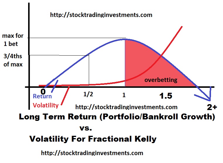
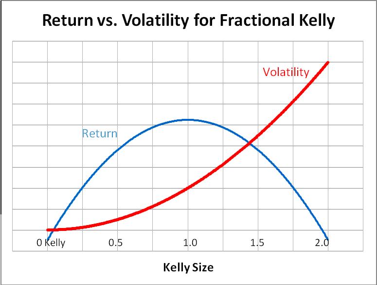
betting more than 2 times the “full kelly” actually turns a profitable strategy unprofitable over ANY time frame, and erases any skill edge you have. While your winners may also compound, your losses create disproportionately large drawdowns that require a greater skill or edge to overcome to get back to even, and due to simple chance those drawdowns are certain to occur over a long enough time horizon with a correlated, unhedged system. Your edge is not as profitable as the expected value calculation in reality, at least not without introducing a “risk of ruin”. But I digress, let’s keep things simple… Pot odds. To keep things simple and ignore “uncertainty”, I want to use a situation in trading which the numbers tend to be a bit more concrete as opposed to uncertainty, so I want to give the example of “risk arbitrage” through buying into mergers and acquisitions.

According to this blog entry, 97 deals were completed, only 2 deals failed. However, many others remain unresolved and sometimes it may take longer than anticipated to close which doesn’t eat into your total profits for the trade, but does eat into your annualized profits since it takes longer for you to be able to reuse that capital. Since we are concerned in this article about profitability and pot odds, time will not be factored in. Even though almost 98% of deals closed, we will leave a bit more margin of error since some deals can linger on for years and then not close which could skew the numbers a bit. To be safe, we will say over 90% of deals go through and we can say that with pretty substantial confidence. At 90% chance of being right to win X and 10% chance to be wrong and lose 100% we must solve for X such that -.9x=-1*.10 or.9x=-.1 or -.1/-.9=1/9=.111111=11.1111%.

If you would lose 100% and win 11.111111% when you are right, the strategy of buying into these deals post announcement would be break even. So if you put your entire capital at risk, you would have the “pot odds” to buy any time there is a 11.11% payout or better. But when deals fail, they don’t go to zero, they drop down to around their pre-buyout price on average. This can change from deal to deal and some deals may just be in a constant downtrend.

If you had a downside of only 10% and an upside of only 5%, how would it compare with a trade with a downside of 100% and upside of 20%? You can confirm the expected value by downside of a loss (expressed as negative percentage) times probability of a loss plus upside of gain plus probability of a gain.

System 1 10% downside, 5% upside:

(-.1*.1)+(.05*.9)=.035=3.5% per completed deal.

(-.1*.1)+(.2*.9)=.08 or 8% per completed deal.

This shows why I don’t like expected value in comparing two systems, you risk insolvency by putting 100% of your capital into the trade with the “higher expected value” where as you only put 10% of your account at risk with the “lower expected value trade” If you were to risk 10% of capital on the 2nd strategy, you would only grow your portfolio by 0.80% per deal. As such the deal providing the better risk reward assuming equal probabilities of success/failure is almost always going to provide the better return on risk. You must evaluate system on an equal portfolio risk basis to truely determine which is better. The kelly criterion is a good metric for comparing one system to another on an equal risk basis. However, the kelly criterion should not be used for position sizing as it is probably 5 times more aggressive than it should be (or more) due to the false assumptions the formula makes about having an “infinite time frame”, a “certain, predefined known edge” and “complete emotional tolerance for all volatility that does not effect your edge” and that multiple bets at a lower percentage with a low correlation provides a better return on risk overall.

Additionally, if you could complete 12 trades a year in the 3.5% expected value system and the  8% per deal system took over a year, it would be much more profitable, so a raw calculation of “expected value per trade” must first be “normalized” (in this case normalized means something very different than “normalizing” volatility” as instead it means it should be set up to reflect the “normalized rate of return at a given level of risk” to reflect overall growth on portfolio given equal risk via position sizing). Then it must be also “annualized” so that they are equalized on a particular time frame after fees… However, due to uncertainty, you also must consider that the large edge that compounds fewer times is less vulnerable to small changes that may negatively impact the ROI more than you thought.

I don’t want to get any more complicated than I already have in this article, but for now I will tell you to practice by looking at your “risk” and your “reward” and measuring out your probabilities required to break even. For example if you have a target price that nets 3 times your risk, you need to hit your target 1/4 times in order to break even.  With options if you try to hit around “break even” on hitting your targets or even lower, the trades that expire in the money and have to be sold for a slight gain, break even and only a slight loss as opposed to the entire risk of the option PLUS the occasional trade that runs beyond the target will create profitability in the system.  I get into more specific and more realistic trading systems in part 2 and part 3.

Comments »

Equity Curve Of Risk – How Risk Influences Expecations

In the last post I discussed how I used a system and position sizing simulator to look at the ENDING equity of thousands of traders trading a theoretical system. I mentioned I would be showing sample equity curves at a given amount of risk by pulling up a random trader. It’s a lot easier on the spreadsheet to get a better sense as you can just press the F9 key to recalculate the random iterations and thus instantly bring up an entirely new random equity curve with all the same settings. You can go through several examples in a short amount of time. It is a bit more time consuming to create new JPEG images of each of them and then post them here so I will only be showing a few.

To further illustrate the type of “risk” you are taking by a particular strategy I provide just one random “trader’s” equity curve of each of them. Understand that results may not be entirely typical but pay attention to the % drawdowns to get a broad sense of the type of risk you may look at and endure.

Please note: The actual expectations of the system you use will drastically impact the type of volatility you see with every 1% change in risk. These sample equity curves are only made with the trading system with an expectation of a 20% chance of each of a 50% loss, 50% gain, no change, 100% loss and 150% gain.

1% risk

1p risk

2% risk

2p risk

5% risk

5p risk

As you increase risk, the results become more polarized and more extreme, so I will provide a few examples for those at the supposed “optimal” risk percentage of 14% risk

14d2 14d 14.2 14

The phenomenal results of a few skew the results of the rest. The drawdowns are insane as you see 70% and 80% drawdowns.

Can you stand 80 trades of being down steadily as your account drives lower to HALF of what it started with? Most people can not and would capitulate so even putting 5% of your capital into this “system” becomes problematic. Granted multiple bets with a lower correlation that adds up to 5% or even more may be actually “lower risk” than 5%. Granted, you can potentially use strategies that actually profit from market overall volatility such as allocation models and rebalancing and modern portfolio theory and hedging and pairs trades and such, you can put in some income and weight a lot of your portfolio with stock that have more of a slow and steady drift upwards that 70% of the time actually provides more stability and increased liquidity that can comba the negative effects of account volatility. Granted, a MORE profitable system can allow you to risk quite a bit more without the same drawdown expectations…. But even so, we are talking about a winning system where even at 1/3rd of what some quants would suggest to be “optimal” over a finite amount of time the returns are very likely to be terrible over a significant period of time.

Can you see why long term capital management went bust now as they did not test their assumptions while taking only a small sliver of time in the past by which to evaluate their “expected risk”?

I could get into how uncertain the world is and how your estimated “edge” within a system is also not a certainty which is still an assumption that this model must make to provide results, but at least can be recalculated with different sets of expectations. But I hope that this post has been educational enough for you to make at a minimum slight, productive adjustments to your way of thinking, if nothing else.

Don’t blow up like LTCM… Test all of even your most basic assumptions… Evaluate your risk in as many ways as you can. Understand risk and how to manage it. Control your destiny rather than being a victim of your own emotional compulsions to sell at the worst point of time and capitulate just before your system takes off because your system is too volatile. Understand the dynamic nature of reality and how increasingly large leverage and risk may be increasingly more volatile while also being more vulnerable to small changes in the conditions by which you based your assumptions. Understand the need to be well capitalized and that fees aren’t factored in and more negatively impact the volatile systems that have an increased probability of drawing down significantly from the starting point. Constantly seek to let the facts guide your conclusions, and seek productive improvement on the way you look at things. Then risk can serve you, rather than you “getting Serrrrrrved” by risk.


Comments »

How I Let Data Guide My Conclusions and Results Of Thousands Of Monte Carlo Simulated Trades!

I stand to you today to announce that I have used data and simulation to prove myself wrong. Call me a flip flopper if you like, but I view this as a constructive thing as I have chosen to take the most profitable and beneficial path rather than the most comfortable. While some remain attached to certain ideas, I let the data guide my conclusion whenever possible. The human mind is full of biases and often too rigid on our ideas. Be open to examining the assumptions that you take for granted on a daily basis just as testing the assumption that “the world was flat” was a productive one, it is possible you may make significantly greater progress than all of those around you who resist the change in your ideas.

My previous paradigm was guided by this understanding of the relationship of risk:
kellycriterion
Unfortunately, every model has certain “assumptions” it must make to construct any particular generalized “model”. It is usually not the model itself you should test, but the assumptions within the model, as well as your own personal assumptions which can only be done by data first. After adjusting and testing these assumptions and thinking more dynamically I can see that this is simply not practical as you will also see in a bit.

At first I had a simulator created to calculate all possible permutations of theoretical trades, but realized the simulator could be improved. Rather than continuing down the direction I was headed, I “flip-flopped” again, instead opting for constant improvement. I instead came up with a spreadsheet that uses the random number generator and a “Monte Carlo simulator” plugin that I view as much more efficient and flexible in terms of the duration of trades in which I want to test. Although it lacks the same degree of precision, it is a productive tradeoff as you can still increase precision in exchange for a more timely monte carlo simulation (with more random iterations).

I used the spreadsheet to look at returns dynamically over a finite amount of time such as 300 trades. Out of a thousand traders for example, some percentage may gain 20% while another percentage gains 100% and another percentage loses 50%. Using this data, A histogram plotting all simulated results of each of the thousand random iterations of 300 trades was made for various levels of risk given a particular system. The simulation allows for a change of any one of these inputs (probability of 5 different “results” of the trade, the ROI given each of these 5 “results” the number of traders randomly selected and the number of trades they make). You can even look through random equity curves across all 300 trades at a given risk factor and refresh it with a push of a button to pull up another random trader to get a better sense of drawdown within different points of the system over the course of those 300 trades.

Without further ado, here are some results!


results

pX=probability of event X.

wX=win % (ROI) given event X.

System: p1-5=20% W1=150% W2=50% w3=0% w4=-50% w5=-100% A winning system is presented.

Risk defined as capital at risk since this is an option strategy and you can lose the entire premium.

“optimal F % / full kelly = 14% risk”

Note the severe skew right. This means as you increase risk extreme outliers begin to skew the average higher than what is “typical”. Skew right means the mean (average) is way higher than the median (average). The “worst case scenario” grows with risk. The probability that you end with a lower than average result (that is not a typo) increases as risk increases risk given a finite amount of time. Eventually the probability of a poor result is so great that as you increase risk the long term geometric return suffers. If you are a true cowboy looking to become an “outlier” and willing to put in the risk, then perhaps that is okay with you, but just know that going beyond the “optimal” amount is destructive as you approach “an infinite number of trades”. Just know the type of CRAZY account volatility you will have to endure, and a large probability that you actually will end down even after 300 trades. That’s almost 6 years at 1 trade a week!

Since I took the time to create this spreadsheet, I can simulate thousands, or if I like, tens of thousands of traders trading anywhere from 1 to 300 trades (or more if I take 5 minutes to set up more) with a given system with a push of the button. I can instantly adjust the expectations of the trading system and see how the results change.

In the next post Titled “Equity Curve of Risk – How Risk Influences Expectations” I show some example equity curve of a particular risk percentages.


Comments »

Trend Following Strategy Using Sound Money Management Principals

I’ve decided to keep this blog on ibankcoin specific to trends. To keep this blog on topic I made a post at stocktradinginvestments.com titled Kelly Criterion Shows Decreased Correlation Increase Return. The short version is the picture worth a thousand words.
Kelly-Criterion

Reducing correlation (and thus increasing your independence of your bets) is important because you can reduce your draw-down, or increase leverage in multiple uncorrelated names and keep the same draw-down with higher long term returns. If you lose 20% you need 25% gain to make up for it, but if you are invested in uncorrelated assets, a 20% loss will be much smaller as your overall portfolio, even if you have multiple uncorrelated bets with leverage. That is the idea.

What’s this all have to do with trend following?

As great as it would be to go “all in” in the best possible area and get every single call right, that isn’t realistic.
This is why I propose you set minimum holdings for risk on assets (stocks,natural resources&commodities,etc) and minimum for risk off assets (currencies&cash, bonds,). But also consider other lowly correlated opportunities. Depending on the trend, you would adjust your weightings, but not necessarily neglect opportunities if it keeps your portfolio’s correlation low.

When stocks go down when you expect them to go up, if you are 100% invested in stocks you not only are down in your position, but you also lose in opportunity to rebalance at lower prices, and in some extremes even change your allocation to be more aggressive. There is a fine balance between trend following and value investing. Value investing principals would suggest that if you are bullish if a stock is at $100 you should be more bullish if a stock is at $90. Trend following is often, but not always, in conflict with this, especially in individual names vs indices. This means you have to be positioned within a trend both to take advantage of the directional move, and also to take advantage of fluctuations in prices away from the trend (contra-trend moves), and to position more heavily if the signals are stronger. But unless you are 100% certain or the move severely outweighs the downside of it going against you, you do not want to be 100% in any asset class. Additionally because daily and weekly volatility (noise) exists within a monthly trend, it still may be right to have some funds you can transfer, despite also being “right” about trend direction since we still may have opportunities to add stocks lower in a monthly uptrend, or add to TLT or “risk off” trade at a lower price in a monthly downtrend (downtrend in equities, that is). For this reason we set parameters.

So we set parameters of maybe 75% maximum and 25% minimum for both risk off (bonds) and risk on (stocks). (You could certainly go with less or more depending on how you want to push your risk, and maybe make an exception or two). We also want to keep what we learned from the linked to post in mind and make sure an area of low correlation has it’s place.) Having this much is a bit more for longer term traders and contrarians looking to preserve enough cash in the event of a big plunge. If you are more nimble and more accurate go ahead and change this, but the rare times you get caught long in a big decline or vise versa, you will often make up for all the opportunity you missed out prior to the big run. Another solution would be to find more pair trades and hedged positions.

Overall though, you have to not only keep track of the trends in stocks, but in the alternative investments.

To keep things relatively simple, I came up with a general guideline to follow for stocks. I started with defining what type of trend we are in . We can be in 4 trending conditions:

Monthly trend up, weekly trend up

Monthly trend up, weekly trend down

Monthly trend down, weekly trend up

Monthly trend down, weekly trend down

Then I threw in overbought and oversold conditions. Within each of those trending conditions there are 4 possibilities. Either no extremes, weekly extremes, monthly extremes, or both weekly and monthly extremes. This gives us 16 potential scenarios to account for. (In reality there are more because 3/4ths of the trend signals for example can signal an uptrend) If you want to use The PPT OB and OS signals there are 32 potential scenarios.

The simple way is rather than make 16 more adjustments, to just note the 16 conditions first then as a rule of thumb subtract 10% from stocks and add 10% to bonds when PPT OB and -1% from stocks and +1% to bonds every additional 0.1 OB points it gets. And for PPT OS to add 10% to stocks and subtract 10% from bonds and add +1% to stocks -1% to bonds every additional 0.1 OS it gets. A more complicated solution would more aggressively sell the overbought signals and more cautiously buy the oversold signals when weekly trend is down (but not oversold), and more aggressively buy the overbought and more cautiously sell the oversold when weekly trend is up (but not overbought).

Then I went through each condition and came up with a potential allocation. To keep it less complicated I just chose “Arbitrage” as the low correlation play mixed in with “treasury bonds” and “stocks”. In reality, “gold” “natural resources” should be considered for “risk on” plays as well. And “currency”should be added in addition to “bonds” for “risk off” plays. Adding in MORE lowly correlated assets and using leverage when appropriate will increase return without at the expense of volatility and long term growth.

In some conditions, leverage is allowed to be added depending upon the asset class.

Since originally writing this article, I decided to keep an eye on these as a guideline, but to change the individual assets. So the principals remains in tact of what percent is “risk off” asset and what percent is “risk on” and what percentage is “arbitrage” or “minimal correlation” to the rest of the portfolio. But the actual percentages changes based on trend.

As you saw in my most recent post the trend trader, I came up with a sort of “model portfolio” to follow in the current conditions. In reality, I may shift a lot more heavily to arbitrage if the deal is right and I may leverage it if the deal itself does not seem to require leverage. For example, if Apple or Google bought something smaller, they would probably have enough cash on their balance sheets and the concern of the deal going through would not depend on availability of credit. If the economy turns south in a hurry as it is vulnerable to do in a monthly downtrend and weekly downtrend, or monthly downtrend with a weekly overbought condition, deals can fall through, so avoiding leverage, keeping that percentage of your portfolio towards arbitrage small, and being cautious makes a lot of sense. There are those I know who just trade pre earnings both long and short certain names, This would be a pretty low correlation type of trade so “arbitrage” when market isn’t vulnerable to sudden credit contraction and rising LIBOR rates isn’t the only way to have a near 0 correlation, it’s just the one I am going with. Earnings has larger moves in a short period of time and may require greater number of trades at a smaller position size to reduce potential for a large downside swing in portfolio size. What I am trying to communicate here are the PRINCIPALS though…

You can use the trends, or use value weighting or whatever signal you want for adding lower and selling higher via rebalancing, or more aggressively repositioning your allocations. But A very often overlooked goal is how your overall return on risk within a portfolio comes out. And to do that, it requires multiple assets with low correlation weighted towards which ones have a higher probability of equal upside/downside or greater overall edge, and a focus on low correlation. Once you can accomplish that, you can determine your return based upon leverage and how aggressively you position one way or another.

I have another post I will work on that further illustrates this difference in leveraging up your returns vs no leverage given everything else is roughly the same.

Comments »