iBankCoin
Home / Tag Archives: allocation

Tag Archives: allocation

How Many Trades Should You Have At Once?

Ever wondered how increasing the number of trades in a period changes your performance? I’m really close to figuring that out to a very specifically defined calculation. The one missing variable is “correlation”. I don’t know how to account for it and how correlation impacts probability.

So for this experiment we’re going to assume binary outcomes of -100% or +250%. I’m going to assume my own variation of the kelly criterion strategy so I can model them at an equal amount of risk(?).

The logic is: If the maximum you can bet to maximize geometric growth at one single bet is 10%, then after a single bet you are left with 90% of cash. If you lose, you will be making a bet that is 9% of your initial capital anyways, so we can allocate 19% for two trades that we hold simultaneously provided there is zero correlation. If we are going to make a 3rd trade we are 81% cash so we can add an additional 8.1% risk and divide the total amount at risk by 3 and so on. It’s possible you can risk slightly more than 19% for 2 but less than 20% because a loss isn’t guarenteed. We will position as if the first position lost due to the possibility of it losing and the nature of overbetting providing less return at increased risk (where as underbetting provides less risk and return only declines slightly)

Background

For some brief background on how the risk amount to maximize growth, see the Kelly criterion. Essentially you are going to take (O1^N1)*(o2^N2) where O1 is the wealth multiplying outcome at the given position size, and N1 is the number of times you produce that outcome. For instance, at 1% position size with 250% gain and 100% loss for outcomes, O1 is 1.025 because a 1% position producing a 250% gain multiplies  our wealth by 2.5% or a factor of 1.025.

This is calculated by

1+(.01*2.5)=1.025

And the loss is .99 which is calculated by

1+(.01*-1)=.99.

So for 20 wins and 30 losses the equation for how much our wealth changes is (1.025^20)(.99^30).

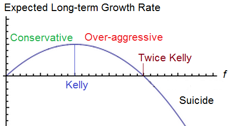
The Kelly criterion reverse engineers the position size to solve for the position size which maximizes geometric rate of return based upon your assumptions over an infinite number of bets. As volatility increases, eventually return decreases. The kelly bet seeks the point at which you can no longer improve the return without much respect for the volatility. In reality, you’d probably wish to respect a fractional kelly strategy if you want to reduce risk. It’s a good way to compare systems at an equal amount of risk. Right now I’m using a modified kelly. It is similar logic as the kelly but not the kelly exactly to increase position size based upon multiple held positions.

You could manually adjust the position size for very large outcomes with a proportional amount of wins and losses until you can’t seem to increase it to approximate the solution, or just use a kelly criterion calculator. You can run more complex calculation with more than 2 outcomes, but for now I’m just using 2.

Optimal Bet Size

So the optimal bet size for a single bet is 9% given 35% chance of a 2.5 to 1 payout.

We can then solve for the optimal bet size for 40 bets assuming zero correlation between trades but with 40 trades held during the same exact time period. There’s an important distinction here. Rather than multiplying our wealth by 1.025 with each win, at this point we are only adding 0.025 to the total portfolio per win because we don’t get the benefits of compounding when the trade is placed. Similarly, if we hold 40 1% positions at once and lose them all, we don’t lose 1-(.99^40)=.331 or 33.1% but instead lose the full 40%. So the first formula is not sufficient in describing what happens to our wealth. This is also where correlation is a bigger liability than the formula currently realizes as the chance of greater drawdowns increases as the correlation increases.

As explained before, we are going to assume a full kelly and then an additional full kelly of risk with the remaining capital for each additional bet. Since the full kelly is 9%, that means the cash on hand remaining is .91 of our portfolio which can be multiplied for each of 40 bets to determine how much cash on hand to keep

or .91^40 to equal 2.3% which leaves 97.7% at risk divided by 40 is 2.4425% per bet.

We can repeat this for 30 bets, 20 bets, 10 bets and 5 bets to construct a table of optimal bet sizes per bet.

Bet size given total number of positions.

50 bets 1.98209% per bet
40 bets 2.44251% per bet
30 bets 3.13649% per bet
20 bets 4.241775% per bet
10 bets 6.105839% per bet
5 bets 7.519357% per bet
1 bet 8.9999999% per bet

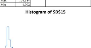
Now we can construct a simulator that sums the total % gained per bet over a period for 12 periods and randomizes the outcome according to the probability.

Excel gives us a function =RAND() which delivers a number between 0 and 1. If that number is less than .35 it will deliver a 2.5 times the position size outcome. If it’s more than .35 it will deliver -1 times the position size as the outcome. All position sizes for a period will be summed up and the number 1 will be added and then multiplied to the portfolio size and then the fees for the period will be subtracted. 12 periods will be simulated giving us a yearly total. We can then run through 1,000 different yearly results and see the distribution of results, the average, and even estimate the compound annual rate of return

This way we can see when the benefits of diversification outweigh the costs for smaller 5 figure portfolios where fees eat into profits. I am probably over estimating fees slightly as I used $6 per trade and assumed buys and sells for all trades, where in reality there is only an opening trade for 100% loss trades.

The CAGR is a crude estimate as the simulator only gives me the first 100 results. I am basically taking the returns plus 1 and multiplying them all and estimating X where X^100 equals 1 minus the multiple factor of the first 100 results. The CAGR will be substantially less than the mean outcome. TO illustrate imagine a 25% average return where the results are -50% of your portfolio and then +100% The actual CAGR of an equal amount of -50% returns as 100% returns would be zero, not 25%. The CAGR reflects the loss due to volatility.

I assumed a 20,000 starting portfolio and $6 fees with the assumption that there was both a buy and a sell order for each trade. Trade fees were deducted after each period’s multiplier was applied.

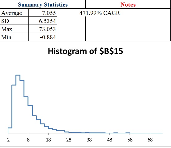
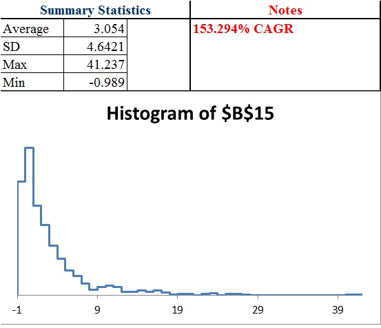
40 trades @ 2.4425% position per bet

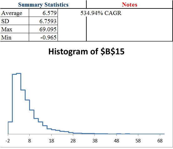
30 trades @ 3.1365% position per bet

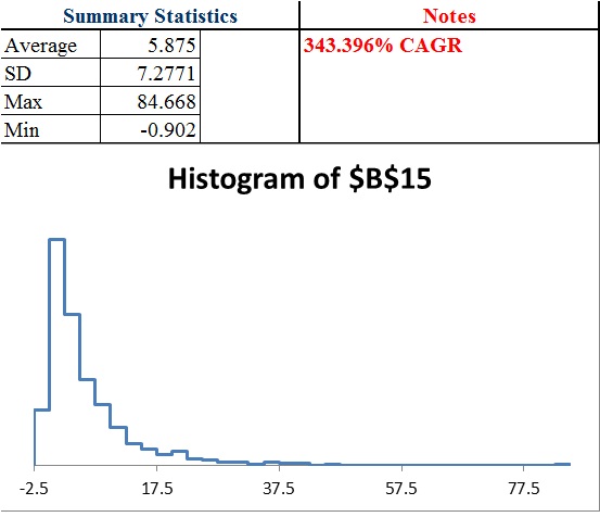
20 trades @ 4.2418% position per bet

15 trades @ 5.0466% position per bet

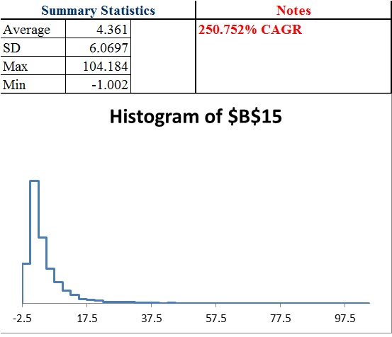
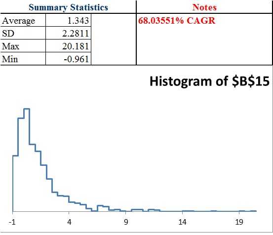
10 trades @ 6.1058% position per bet

5 trades @ 7.5194% position per bet

1 trade @ 9% per bet

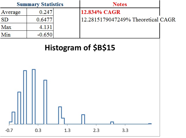
For 12 independent trades or 1 per 1 month period, the theoretical gain is .97% growth per bet or 1.0097^12=~12.28% growth per year… theoretically. But that’s over the time horizon of infinity and as you can see by the distribution should 1,000 traders have the same exact expectation, the actual results over a year can vary wildly. Also, with only a $20,000 account taking too much risk or not enough can result in problems should losses occur early because of the size of trading fees being a flat amount.

We find we can greatly enhance the return by adding more position sizes, but the benefit of diversification decline with each additional bet.

Adjusting For Correlation

While I think the above can give you good idea for how many trades for a given portfolio size you should hold at once (and we could easily adjust the calculation for half of the initial kelly bet), we still have yet to develop a system that adjusts bet size based upon correlation. What I believe is true is that as correlation approaches one, the total amount risked should approach the single kelly bet. Afterall, if you bet all your capital on multiple trades of the same coinflip, it would be no different than betting a single bet on that coinflip. In other words in our previous example as the correlation increases the total amount at risk should approach 9%. This means that the ideal bet in reality is somewhere between the bet size calculated above at the correlation at zero (that has been calculated as shown in the prior table) and the correlation of 1 which is 9% divided by the number of bets.

For instance, if the correlation was 0.50 across 20 bets.
A correlation of zero suggests [1-(.91^20)]/20=4.241775% per bet.
A correlation of 1 suggests 9%/20=.0045 or 0.45%
Since the correlation of 0.50 is the midpoint between 0 and 1 we can average the 2 and get 2.35%*

*but that’s only an approximation.

Unfortunately the relationship may not be linear, so while we can be sure the optimal bet size for maximizing CAGR across 20 simultaneously held bets is somewhere between 0.45% and 4.241775%, we can’t be sure it is the exact average of 0.0234589 or ~2.35% per bet.

I also want to look at “half kelly” strategies in 2 different ways. One is dividing the per trade bet by 2. So for 40 bets if we calculated 2.44% the half kelly could be 1.22% per trade. That halfs the total amount of capital at risk. The other is using a 4.5% number initially, and so a 0.955^40=~15.85% cash on hand or ~84.15% invested divided by 40 or 2.10365% per trade instead of 2.44%. We can see that that is still much more aggressive than halving the amount per bet.

Normally the half kelly solution provides 3/4ths the return at 50% of the volatility of the full kelly. This is really promising for multiple bets when we can reduce the amount at risked by only a small amount and still be at an equivilent of a half kelly strategy in some regards.

In the future I also want to come up with a different calculation such as solving for the “probability of a 50% decline or more in a year” (or probability of 100% gain for example). This is pretty easy to set up.

If the result is -50% or less in a year, a simple formula will give me a 1. Otherwise zero. The average is the probability of this event. This helps you better model the probability of achieving a certain result (such as 100% return) while measuring it against a probability of a negative outcome (such as 50% loss) so you have a different way to compare risk and reward of position size and number of trades and understand expectations.

For now it seems more bets is better up to a certain point where the quality of opportunities and expectations as well as the fees become problematic. It’s hard to identify where that is, even with thousands of simulations because of the increased “skew” (the expectations become increasingly dependent upon a smaller and smaller probability of a more and more spectacular outcome) as risk and number of trades increases. Also, as your bet size decreases the aggressiveness and increases the amount of trades, the fees should become more problematic which I think we will see in a half kelly and 1/4th kelly simulation. Lowering your position below 0.50% when you have a $20,000 portfolio for example might become a problem and eat into returns too much. As such as we seek to decrease our risk, we will eventually have to decrease our number of trades or else position size will be too small given the fees to provide as big of an edge.

Comments »

Asset Allocation Strategy

PP

Capital has to move. I believe the market can almost never be in a state of equilibrium because new debt is being created which creates additional capital that changes the balance of allocation, and old debt is being replaced when it’s being paid or assets are being foreclosed for the inability to pay and moey leaves the system or rotates away from one particular system such as a domestic, localized economy to a foreign one.

As such, the efficient market hypothesis can almost never be exactly correct, and if it could be, it only is for a moment since new debt being created and old debt coming due and interest payments are never coordinated to sustain parody in the market place. People have to make moey to pay bills and transactions HAVE to occur. If they don’t, such as in communism, the economy collapses as has occurred historically anytime any nation even attempts to move towards a communistic state.

With this in mind, we still should care about how one might position in an effecient market, because a true “game theoretic optimal solution” or “equilibrium solution” is indifferent to how the actual market is positioned. The key behind this philosophy is to position such that you profit from a movement of capital regardless of in which way it occurs.

A simplified example is shown at the top of this post, but an even more simple one would be a world where you could choose between 2 types of currency assuming neither could be eliminated from legal usage. The optimal “equilibrium” solution would be 50% of each at all times. If 99.9% of the world used dollars, you still would gain from 50% mixture of each because you’d maintain the ability to reduce higher and add lower. If it was 99% the other way that would also be the case. Although a more “exploitative” solution would be to position the inverse of the crowd such as being 99.9% of the currency that is owned by .1% of the population, that doesn’t detract from the profitability of the “equilibrium” solution of 50/50%

Understand this difference because I do not advocate an “equilibrium strategy” entirely, but by being aware of it you can deviate from it to the degree by which you have an edge and to the degree by which you can stand volatility.

If you have an edge, you can try to assess that edge probabilistically and use simulations to match your goals such that you have an expectation that satisfies you at a level of volatility that you can stand.

If you were to integrate your ability to make short and long term trades, you might create a baseline that adds in an edge playing the market, but curbs it with an allocation based equilibrium strategy as a core staple of that strategy in the following regard.

equal

As you can see, by including individual short term and long term trades as an allocation, there is a bias towards stocks and stock picking.

With the introduction of this, the problem is that over time your allocations will change and the reality of transaction fees require less frequent rebalancing. Also, individual trades usually have upside expectations and you want to let your winners run. As such it is possible that your individual positions may cause portfolio to grow out of balance. So you probably want to build in a more flexible mechanism to maintain overall parody with regards to your intended allocation of risk and stocks overall. This can be demonstrated below
1

2

3

Rather than sell short of targets to maintain balance in asset allocation, you can use this reflexive, adaptive model to maintain the balance. As long term allocation grows you can reduce or entirely sell your broadbased stock ETFs. As short term allocation grows you can add hedges that last at least until your exit strategy triggers a sell and the increase in cash can allow you to make the adjustment to bring your strategy back into the intended risk allocations. You can develop more complex models to work subasset class allocations as well, and even try to handicap those or handicap the actual market movements by weighting your positioning according to risk and reward and expectations overall to more aggressively try to game the market as well as use leverage.

4

If you believe that you have a large enough edge and want to use additional information, you may use volatility as a tool and include options.

When volatility is high, you add to option selling strategies or XIV or SVXY ownership, and you might add to broadbased ETFs since correlation tends to be higher and the edge for picking stocks is less. You might increase longer term exposure following a crash weighting heavier in value and fundamentals. When volatility is low, you add to overall option exposure and may opt to reduce your allocation of XIV or SVXY. When correlations are less you may want to increase option ownership and decrease broadbased ETF ownership and look to apply your “edge seeking” as a larger percentage of your allocation.

This dynamic approach can still have with it a set of rules from which to govern the overall intent, and some kind of checklist to help you operate it efficiently as intended. The overall idea is to not get emotional and allocate emotionally, but instead strategically according to a plan made when your mind is operating at a high level, rather than when you are in fight or flight mode and you’re in “panic mode” and your amygdala is active.

So if I were trying to game the market right now, on the long term I may be interested in commodities, but in the short term I don’t see any setups. Any allocation towards ETFs or calls would have to be with plans of long term ownership. I think it’s a good entry for a longer term horizon on the stock market, but the individual names aren’t suppolying great entries aside from maybe some long term stock investments.

So with a volatility spike I’m rotating out of my individual stock trades as they stop out, and then if I have any hedges, I’m seriously reducing or taking them off as the decline reaches extreme. I’m looking on adding or increasing an inverse volatility ETF as long as the primary bull market thesis remains intact, and I’m looking to position for long term stocks but I’m not really looking to add long option strategies. I may be willing to sell puts on stocks I’m willing to buy or sell put spreads on stocks with high IV that look to be likely to hold or go higher.

You don’t necessarily need to force trades, but if you have thought all of this out and have thought out position size, maximum and minimum allocation for each assetclass or a way to objectively determine the allocation based upon certain measures, you will avoid fear taking over.

You will also be able to remain consistent. One of the biggest problems traders run into is that at the bottom, an allocation of 50% stocks seems high, where as at the top it seems low… At the bottom finding individual stocks to buy is tough, where as at the top they are easy. This is why you need a system in place while you’re thinking rationally that you can apply as the market changes, or at least increase the size of your hedges and bearish bets at the “top” while selling you broadbased ETFs to counterbalance your ability to have confidence with individual positions without unnecessarily over exposing yourself.

You also need to have thresholds at which you rebalance. Perhaps if a stock is within 5% of targeted allocation you don’t bother rebalancing, but outside of that number you do.

from an exploitative philosophy it’s okay to increase your allocation as the market goes lower if you are buying individual stocks, and you have some sort of risk management mechanism which acts as a kill switch if buying lower fails. While in equilibrium strategy you don’t want to expose yourself to further declines with a “martingale” type of strategy, there are many times when both the odds of a bounce and the expectation when it does happen actually increases as stocks get more oversold. But you need to have limits. So if your average allocation of an asset class is 25% you might take that up to a maximum of 40% when buying the ideal oversold conditions and down to 10% or 5% when selling oversold.

I can’t define these to you because that depends upon what your pain tolerance is and what your goals are and timeframe for those goals, and whether or not that is realistic for you.

With an equilibrium strategy, you are basically looking at a strategy that works over an infinite time horizon, where as realistically you should approach it with variance in mind. As such, position sizing becomes important and your cash position should increase. This is why the logic to weighting assets by volatility may actually make some sense on the surface, but I don’t believe it’s pure equilibrium strategy.

Unfortunately, that which is not volatile may not remain that way forever. I believe real estate had not undergone much downside volatility at all for decades until it finally crashed in 2007-2009. The global demand for bonds on the basis that it has been “safe” or less volatile isn’t an accurate reflection of the last 200 years of history where governments defaulted, nations have risen and fallen and political power and influence has shifted. It may provide some normalization of risk through the INCOME, but that doesn’t make it immune from default risk or loss of confidence and asset class wide loss of risk appetite. Since that risk still exists, you have to ask yourself if the prospect of complete default is worth such a low yield. For example, a 2% yield requires 36 years of interest accumulation until it makes a 100% return. If the chances of a default in that time period is greater than 50% than there is no advantage at all from holding bonds instead of just cash. In fact, it’s worse to hold bonds probably even if those odds were 40% because of volatility risk, opportunity costs of not being invested elsewhere, taxes on income and “black swan” risk even though there are some advantages in curbing volatility as a result of income. For many people even if that amount were 20% due to risk tolerance and transaction costs it may be better to hold cash than bonds, and even if it were much lower it’s not a huge loss. In some cases bonds can be used as collateral to borrow from to create leverage.

The real risk to cash is not the failure to return value, but the failure to protect purchasing power. As such, assets that gain from inflationary pressures, particular that effect the individual the most (such as food and fuel and stocks) is the best way to mitigate that risk. Currently, I don’t view a shift of capital from stocks to bonds as a major risk to stocks, so overall the exploitative strategy should probably be to have a mixture of cash stocks, some commodities and perhaps even betting against bonds and finding other income strategies such as preferred shares, corporate debt and occasional option selling strategies when conditions warrant it.


update:

Another approach to maximizing a particular expectation of return is looking at synergy between asset classes. Since the rotation of one into the rotation of another produces gains to the degree at which you are able to effectively buy low and sell high and since allocation of income provides additional capital to more efficiently rebalance and normalize returns, you can look at the downside deviation or the overall deviation of results to compare the overall portfolio strategy as a measurement of risk.

While this only tells you a backwards looking result of how volatility can be smoothed, it is more appropriate than backtesting of actual results since it’s looking at historical correlation.

I came up with the following strategy as an effective means historically to balance risk efficiently as can be seen at this link.

Sortino ratio: 3.23

Sharpe ratio: .87

CAGR: 10.23%

Std Deviation: 8.08%

worst year -2.71%

Backtested since 1985


Allocation:

Intermediate term treasuries 29% (IEF)
Long term treasuries 41% (TLT)
Small Cap Value 11% (IWN)
Mid Cap Value 14%
Large Cap Growth 5%

Midcap values weren’t around before 1985 so the following is the best I could do backtested since 1972.

Sortino Ratio 2.21

Sharpe ratio .76

CAGR 9.81%

std deviation 6.18

worst year -1.67%

10% Small Cap Value
12% Int Small Cap
70% Intermediate term treasuries
8% gold

Another strategy which involves cash to reduce the volatility is
8% small cap value
11% int small cap
3% LT treasuries
47% intermediate term treasuries
24% cash/money market
7% gold

If you progress towards using leverage and rebalancing more frequently, you are going to have to increase cash position and income positions to replenish that cash position so you can normalize the volatility without having to pay a lot of extra transaction costs to rebalance.

Since the goal is not return overall but instead return vs downside volatility, you potentially could leverage this up significantly and still have less volatility than a non leveraged strategy that was more aggressively allocated. The result can be a better return on better risk.

I believe this philosophy is somewhat flawed since it looks at past performance and past risk as defined by volatility and past correlation to determine overall portfolio volatility. I think to some degree, the less volatility a market has experienced over the past the more vulnerable it is to more dramatic volatility if people are following models expecting the future to resemble the past. Once it starts producing more volatility than expected, that forces people to re-calibrate their models and reduce allocation which creates more selling pressure and more re-calibration among mutual fund managers and others.

But I think you can still look at bonds and convert that to other forms of income that are currently better positioned, and try to identify the areas better positioned for growth in the future as well and keep in mind how down years of stock and bonds may see positive results in gold and commodities and how certain assets compliment each other. Or you can use some mixture of a more balanced strategy that allocates among a few asset classes evenly and this mixed with some tweaking based upon your outlook and adding cash as necessary or leveraging as necessary to better meet your goals and risk tolerance.

This is designed to get you thinking about how capital flowing from one asset class to another plus past history vs future potntial and your own volatility tolerance to come up with a flexible strategy that works for you and isn’t overly complicated to follow.

Comments »