In a basic “pot odds” calculation as described in the last post trading systems: pot odds and trading, if you can let your winners run so that you sell your option for 4 times the cost, netting 3 times your risk or 300%, you are getting 3:1 and thus only have to be right more than 1/4. (lose 3, win on 3 the 4th time and break even). However, options are more complicated than that. While you may be right or wrong on whether the stock goes to a price such that you earn 300%, the stock could reach the target earlier, in which case you may make more than 300%. Also, the timing could be late but direction still right, or the stock could gap up or run past the target and exceed your return. As a result, you might have a number of outcomes ranging between the extreme 1000% or so outlier trades to 0% depending on your ability to let the winner run and your tolerance for volatility. A simple pot odds calculation becomes tricky for determining whether or not the system is profitable, and how much. For this you can use “expected value”, but that really doesn’t grasp the expectancy of the system per trade over time. Nevertheless, since 1% risk represents a small amount of capital lost through volatility, it can still be looked at from the concept of how many 1% position trades are taken per year, and you can approximate that the growthrate that occurs in your portfolio is close to 1% of the expected value of the system as a decent starting point. With such a position size, you can take more trades on at once and as a result the gains can compound faster. There is still some correlation (a LOT of correlation during a significant correlated selloff), but by diversifying trades over multiple time frames and spreading out your purcahses and using the occasional hedge, you can mitigate the cost of volatility at very little cost to your overall results.
So let’s get into an example. Say you average out all your trades over 100%, You average all those over 30%, all those between -30 and 30% and all those from -30 to -90% and then all trades that lose more than 90%. That gives you 5 averages that can define your system in the total average of “large wins” “moderate wins” “break even” “salvaged premium” and “full loss”. The frequency of each event determines a number of trades out of all trades. Simply divide the number of trades by all trades for each of the 5 and you have an estimated probability of the return. Average the return of all trades in each category to get the average return.
From here I actually like to model my results as opposed to using expected value, but let’s just give an example:
Last year’s 2013 results before I booked a couple of large wins in TWTR and TSLA were
17% of trades averaged 294%, 20% of trades averaged 53%, 15.8% of trades averaged -1% 23.2% of trades averaged -63% and 24% of trades I rounded down to the full 100% loss.
To do an “expected value” calculation, you simply multiply the probability of each event by the return and then add them together. So (.17*2.94)+(.2*.53)+(.158*-.01)+(.232*-.632)+(.24*-1)=.217596=~21.76% gain per option trade. By letting the winners run in 2014 from Jan until Jun before a few large wins in AMZN and PCLN and others, this yield was just above 40% but it was also substantially helped by a few large outliers well over 500% (GMCR,AAPL,etc) . So how does that translate to portfolio growth? There is an easy calculation that can be done if the position size is small.
Let’s put it at 1% risk or 1% of .2176 expectation=.002176% per trade. In other words, we multiply at a factor of 1+.002176 per trade. (1.002176^X)-1=annualized rate of return where X is the number of 1% trades you can place with this system in a year. Make 300 trades and you are looking at about a 1.002176^300=~1.919-1=~.92=92% annualized rate of return.
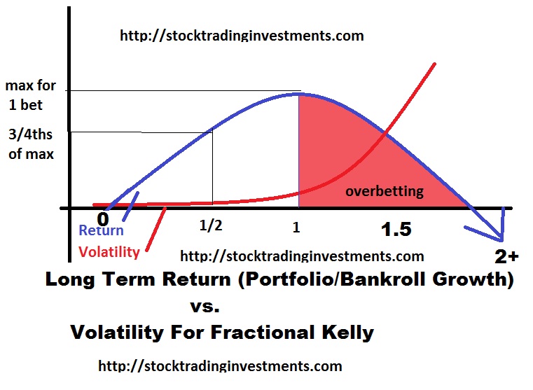
The smaller the position size, the more consistent the system, the lower the correlation between trades, and the greater the edge, the more accurate the estimation is and typically the more consistent the results are with the expectation. However, keep in mind the relationship of return and risk as you look at how it becomes less accurate with increased position size. The assumption that increasing the risk will proportionally increase the volatility and the reward assumes a linear relationship which is not true. Instead the relationship looks as follows:
Nevertheless, we can use a monte carlo simulation to pull a random number between 0 and 1. Since there is a 17% chance of the upper result if it pulls a 0.17 or less, this corresponds to the 294% return result occuring, where as a 20% chance of a 53% return corresponds to a .17 to .37 being pulled and so on. That can allow us to randomly pull the results of a thousand trades, and then through a monte carlo simulation tool we can simulate thousands of trials of 1000 trades and model any particular result or formula as a consequence of each result to get the intended information we need and reflect the results we want. Just by using the average return and ignoring the substantial probability of effective ruin
At 1% with ZERO fees, we get an average return of 91.35% compared to our expected 91.9%
With 2% with zero fees we get an average return of 265.7% compared to an expected ((2*0.002176)+1)^300=268%. Being able to place the same volume of trades as the risk gets too much larger becomes increasingly difficult and increases the correlation risk that is not modeled here but will negatively effect returns. As we increase the position size the difference between the average simulated return and the calculated return grow as the simulation is less and less close to the calculated returns due to losses from volatility. The other thing is, as bet size increased it becomes increasingly difficult to place the same number of trades per year.
What this growing difference does not show is the increasing skew of results. In other words, if 1000 traders were to trade this system over 300 trades at a fixed position size, a smaller and smaller percentage of traders would have a greater and greater result as position size increased. The magnitude of the outliers would increase which would skew the AVERAGE expected results. The opposite side of it would be an increasing probability of poor results as well.
The kelly criterion is a risk management based mathematical formula to assess risk management to maximize gain. Effectively, the more you increase the position size the more you turn it into a lotto ticket, until you eventually take your skill edge out of it and your results actually begin to decline and eventually even become negative if you get too carried away. Even if you are adjusting the percentage risked, you should never go over the full kelly, and since you don’t have an unlimited amount of time to recover the drawdown, and you can only place a few hundred trades per year with overlapping correlation, and there is greater uncertainty… I would absolutely drastically reduce the bet from the kelly. Calculating the “kelly” is a process that has many applications and is another story for another time.
If you enjoy the content at iBankCoin, please follow us on Twitter