3 High Tight Flags for Wednesday

Comments »

For an ETF asset class rotational system which uses weekly data, what is the optimum number of weeks to look-back in order to calculate the relative strength score?

Previous posts on the development of this system.

For this area of development, I set out to determine how robust the weekly look-back periods were. Also, I wanted to determine if there were any benefit to using more than one relative strength calculation. For example, would there be any benefit to ranking the ETFs based on the last ((X weeks + Y weeks)/2) average? Many rotational systems seem to use more than one calculation for relative strength. My gut feeling was that it may be unnecessary to do so.

Based on the results of the last post, the system will only trade on Thursdays. Because the ETFs are ranked using a weekly calculation, there is a delay between the ranking (which occurs at the close of the previous Friday) and the actual trade. I am not sure whether this factor hurts or helps performance. In future tests, I will remove the trade on Thursday only requirement so that the rotations are taking place on the same day as the ranking. In real life, it will be almost impossible for me to trade the system when it ranks and rotates on the same day.

The Rules:

• Buy 1 of 5 ETF asset classes at Thursday’s close based on its X week relative strength rank. Simply put, but the ETF that has gained the most over the last X weeks compared to the other ETFs.
• Re-rank at Friday’s close and rotate or not into the top ranked ETF next Thursday

No commissions or slippage included. Tests run from 1.1.2003 – 3.23.2012.

The Results:

These results show a large area of returns > 10% and drawdowns averaging -25%. I like a period of anywhere between 14 and 20 weeks. Keep in mind that in these tests there is no moving average filter applied to reduce drawdowns.

I chose 17 weeks as the optimum look-back.

Now, lets add a second relative strength rank. Since the first rank used 1-24 weeks, the 2nd one will use 25-52 weeks. This test will rank the ETFs this way: (17_week_change + Y_week_change)/2.

After adding a 2nd calculation and averaging it with the 1st in order to rank the ETFs, we see performance has decreased slightly while drawdowns have increased significantly.

Based on this simple test, there does not appear to be any benefit to adding more than one ranking routine.

Thoughts and Caveats:

Perhaps adding multiple ranking routines makes the system more robust. My results, using only 1 ranking routine, appear robust. There have been many studies which show that a relative strength calculation between 3 to 12 months is robust. 17 weeks works out to be near 4 months. Based on my review of many other studies and the results above, I do not believe it is necessary to use more than one ranking routine.

The ETFs used do not have much history. DBC and VEU did not start trading until 2006 and 2007, respectively. Results previous to 2006 were generated only from trading VTI, IYR, and IEF. This is a rather severe limitation.

These tests are very simple. The idea is to control for each variable, studying the effects, in order to develop a deep and thorough understanding of what makes the system tick.

The next factor to study will be the addition of a moving average filter in an attempt to reduce drawdowns.

Below is the equity curve using a 17 week ranking, holding the top ETF, with all trades taking place on Thursdays.

Comments »

This indicator, designed to delineate the long-term trend, may have finally escaped months of whip-saw action.

Note that the blue line (ROC252) is elevated farther above the red line (ROC5) than it has been in over 7 months.

Backtesting this indicator over all SPY history returns an annualized gain of 11.56%. If traded long only, it returns an annualized gain of 9.13% with a maximum drawdown of -19%.

Below is the equity curve of the indicator trading only the long signals.

It may be hard to believe, but we could be witnessing the start of a long bull market.

Comments »

BONT

SHLD

TUDO

MNTG

TEAR

I’ll update the post later this morning to hyper-link the symbols…Have a great day!

Comments »

Behind the scenes, I’m working on an Asset Class ETF Rotational Model which rotates weekly. This post will explore one aspect of building this model: Which day of the week is the best day on which to rotate?

Using Faber’s TAA as a rough guide, I’ve selected 5 ETFs with which to use for testing a weekly rotational model.

• VTI  Vanguard Total Stock Market
• VEU Vanguard FTSE All-World Ex- U.S.
• DBC  Power Shares DB Commodity Index Tracking
• IYR  iShares Dow Jones U.S. Real Estate Index
• IEF   iShares Barclays 7-10 Year Treasury Bond

One of my earliest thoughts about this system was wondering whether there was a particular day of the week on which to rotate that would be better than the others. It appears there is.

The Rules:

• Buy the ETF on Monday’s close and sell at the close 5 trading days (1 week) later.
• Repeat for each day of the week.

No commissions or slippage were included. All available history for the ETFs was used.

The Results:

Thoughts and Caveats:

If you had to rotate on a particular day of the week and may only hold the trade for a week, on which day(s) would you rotate? On which day(s) would you definitely not want to rotate?

There are no guarantees that this pattern will persist, but IYR and VTI have more than a decade’s worth of history.

If the pattern does persist, rotating on the best day could add enough of an edge to cover commissions or even the expense ratio of the ETFs.

I’m curious what the results would be if the hold time was extended to 2, 3, or even more weeks. Would the anomaly still persist over a longer time frame?

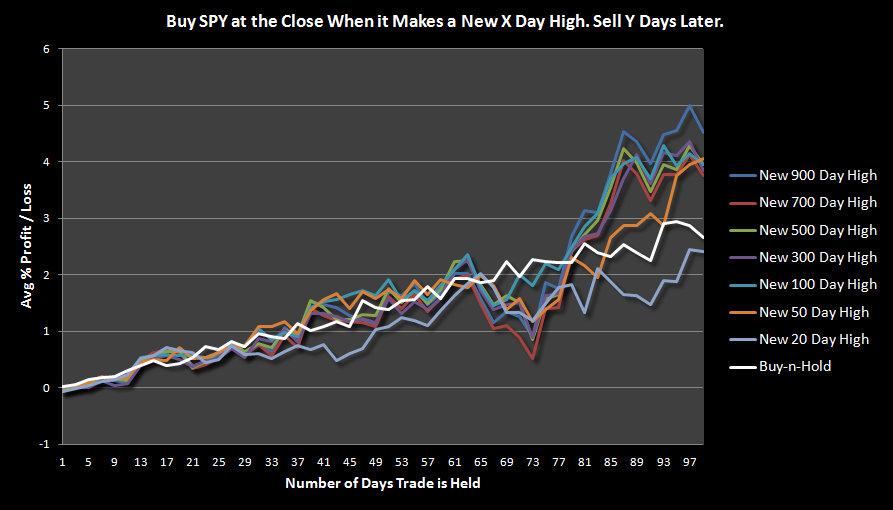
Comments »

On Thursday, March 15th, the S&P 500 made a new 900 day high. With the S&P 500 re-visiting prices it hasn’t seen in almost 5 years, I thought it would be interesting to look at what happens after the index makes significant new highs.

The Rules:

Buy SPY at the close if

• SPY closes at a new X day high

Sell SPY at the close Y days later.

No commissions or slippage included. All SPY history used.

The Results:

Thoughts and Caveats:

Because the market was making significant new highs in October of 2007, the results show the impact of the bear market, starting around day 65. As the trades are being held for 100 days, any trade initiated in October 2007 was held through the beginning of 2008. Ouch.

On the brighter side, a new high of 50 days or greater has seen a surge during the last 25 days of the holding period. This surge appears to be the relatively normal result of buying during a bull market.

It should be noted that a new 900 day high generated the highest return.

Sample size grew as the X day new high number decreased.

The Buy-n-Hold return was calculated by chopping SPY performance into 100 day segments and then averaging those segments.

The bottom line is that save for a new Armageddon a la 2008, the market has tended to keep climbing after making a significant new high.

 

Comments »

A market that does the opposite of what it is supposed to do should is telling you something. Our current market has almost over-extended itself into abnormality. Let’s look at what happens with SPY when it extends itself above the upper Bollinger Band.

Traders must develop abnormal market filters. These filters can be used to denote markets that are abnormally bullish or bearish and will help traders know when trends may extend themselves for longer than normal without a significant correction or pullback. My favorite go-to abnormally bullish market filter is the upper Bollinger Band, set to a 50 day period and 2 standard deviations (50,2).

SPY has closed just 12 pennies beneath the upper Bollinger Band. Although the close is technically beneath the band, one shouldn’t take a completely binary approach to determining an abnormal market. In this case, like hand grenades, close enough counts. Bears who are looking for a swift and sure pullback for this over-extended market may end up waiting longer than they can bear.

The Rules:

Buy SPY at the Close if

• SPY closes above its upper Bollinger Band (50,2);

Sell X days later. No commissions or slippage included. All SPY history used.

The Results:

Thoughts and Caveats:

Results over the first 30 trading days tend to under-perform.

The under-performance or consolidation (compared to buy-n-hold) that is typical after a close above the upper Bollinger Band probably lulls bears into a false sense of security. Rather than putting in a large pullback, SPY has tended to shoot higher.

After getting abnormally overextended,  bullishness tends to persist. This concept is a simple illustration of the power of momentum. During abnormally bearish markets, price tends to slide down the lower Bollinger Band (see SPY in 2008) while in abnormally bullish markets, price will ride the upper Bollinger Band. The chart below shows many examples of this phenomenon.

There are enough samples of this setup for the results to be generalizable.

To read previous posts on both abnormally bullish and abnormally bearish markets, go here.

The above chart illustrates the tendency of SPY to ride up and slide down the upper and lower Bollinger Bands.

Comments »