Ever wondered how increasing the number of trades in a period changes your performance? I’m really close to figuring that out to a very specifically defined calculation. The one missing variable is “correlation”. I don’t know how to account for it and how correlation impacts probability.

So for this experiment we’re going to assume binary outcomes of -100% or +250%. I’m going to assume my own variation of the kelly criterion strategy so I can model them at an equal amount of risk(?).

The logic is: If the maximum you can bet to maximize geometric growth at one single bet is 10%, then after a single bet you are left with 90% of cash. If you lose, you will be making a bet that is 9% of your initial capital anyways, so we can allocate 19% for two trades that we hold simultaneously provided there is zero correlation. If we are going to make a 3rd trade we are 81% cash so we can add an additional 8.1% risk and divide the total amount at risk by 3 and so on. It’s possible you can risk slightly more than 19% for 2 but less than 20% because a loss isn’t guarenteed. We will position as if the first position lost due to the possibility of it losing and the nature of overbetting providing less return at increased risk (where as underbetting provides less risk and return only declines slightly)

Background

For some brief background on how the risk amount to maximize growth, see the Kelly criterion. Essentially you are going to take (O1^N1)*(o2^N2) where O1 is the wealth multiplying outcome at the given position size, and N1 is the number of times you produce that outcome. For instance, at 1% position size with 250% gain and 100% loss for outcomes, O1 is 1.025 because a 1% position producing a 250% gain multiplies  our wealth by 2.5% or a factor of 1.025.

This is calculated by

1+(.01*2.5)=1.025

And the loss is .99 which is calculated by

1+(.01*-1)=.99.

So for 20 wins and 30 losses the equation for how much our wealth changes is (1.025^20)(.99^30).

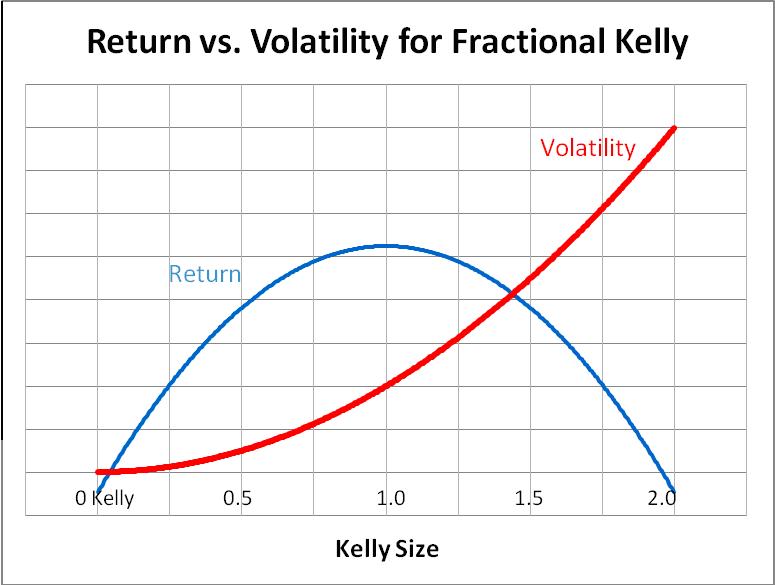
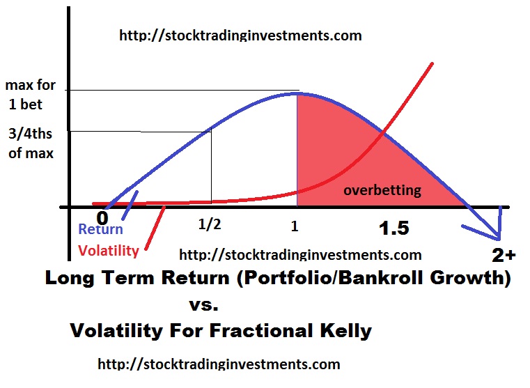
The Kelly criterion reverse engineers the position size to solve for the position size which maximizes geometric rate of return based upon your assumptions over an infinite number of bets. As volatility increases, eventually return decreases. The kelly bet seeks the point at which you can no longer improve the return without much respect for the volatility. In reality, you’d probably wish to respect a fractional kelly strategy if you want to reduce risk. It’s a good way to compare systems at an equal amount of risk. Right now I’m using a modified kelly. It is similar logic as the kelly but not the kelly exactly to increase position size based upon multiple held positions.

You could manually adjust the position size for very large outcomes with a proportional amount of wins and losses until you can’t seem to increase it to approximate the solution, or just use a kelly criterion calculator. You can run more complex calculation with more than 2 outcomes, but for now I’m just using 2.

Optimal Bet Size

So the optimal bet size for a single bet is 9% given 35% chance of a 2.5 to 1 payout.

We can then solve for the optimal bet size for 40 bets assuming zero correlation between trades but with 40 trades held during the same exact time period. There’s an important distinction here. Rather than multiplying our wealth by 1.025 with each win, at this point we are only adding 0.025 to the total portfolio per win because we don’t get the benefits of compounding when the trade is placed. Similarly, if we hold 40 1% positions at once and lose them all, we don’t lose 1-(.99^40)=.331 or 33.1% but instead lose the full 40%. So the first formula is not sufficient in describing what happens to our wealth. This is also where correlation is a bigger liability than the formula currently realizes as the chance of greater drawdowns increases as the correlation increases.

As explained before, we are going to assume a full kelly and then an additional full kelly of risk with the remaining capital for each additional bet. Since the full kelly is 9%, that means the cash on hand remaining is .91 of our portfolio which can be multiplied for each of 40 bets to determine how much cash on hand to keep

or .91^40 to equal 2.3% which leaves 97.7% at risk divided by 40 is 2.4425% per bet.

We can repeat this for 30 bets, 20 bets, 10 bets and 5 bets to construct a table of optimal bet sizes per bet.

Bet size given total number of positions.

50 bets	1.98209% per bet
40 bets	2.44251% per bet
30 bets	3.13649% per bet
20 bets	4.241775% per bet
10 bets	6.105839% per bet
5 bets	7.519357% per bet
1 bet	8.9999999% per bet

Now we can construct a simulator that sums the total % gained per bet over a period for 12 periods and randomizes the outcome according to the probability.

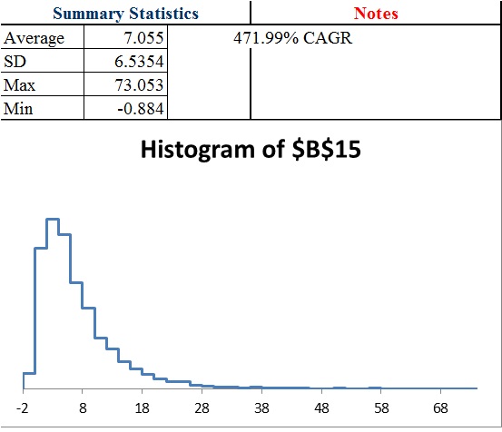
Excel gives us a function =RAND() which delivers a number between 0 and 1. If that number is less than .35 it will deliver a 2.5 times the position size outcome. If it’s more than .35 it will deliver -1 times the position size as the outcome. All position sizes for a period will be summed up and the number 1 will be added and then multiplied to the portfolio size and then the fees for the period will be subtracted. 12 periods will be simulated giving us a yearly total. We can then run through 1,000 different yearly results and see the distribution of results, the average, and even estimate the compound annual rate of return

This way we can see when the benefits of diversification outweigh the costs for smaller 5 figure portfolios where fees eat into profits. I am probably over estimating fees slightly as I used $6 per trade and assumed buys and sells for all trades, where in reality there is only an opening trade for 100% loss trades.

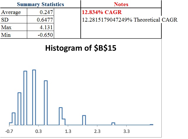
The CAGR is a crude estimate as the simulator only gives me the first 100 results. I am basically taking the returns plus 1 and multiplying them all and estimating X where X^100 equals 1 minus the multiple factor of the first 100 results. The CAGR will be substantially less than the mean outcome. TO illustrate imagine a 25% average return where the results are -50% of your portfolio and then +100% The actual CAGR of an equal amount of -50% returns as 100% returns would be zero, not 25%. The CAGR reflects the loss due to volatility.

I assumed a 20,000 starting portfolio and $6 fees with the assumption that there was both a buy and a sell order for each trade. Trade fees were deducted after each period’s multiplier was applied.

40 trades @ 2.4425% position per bet

30 trades @ 3.1365% position per bet

20 trades @ 4.2418% position per bet

15 trades @ 5.0466% position per bet

10 trades @ 6.1058% position per bet

5 trades @ 7.5194% position per bet

1 trade @ 9% per bet

For 12 independent trades or 1 per 1 month period, the theoretical gain is .97% growth per bet or 1.0097^12=~12.28% growth per year… theoretically. But that’s over the time horizon of infinity and as you can see by the distribution should 1,000 traders have the same exact expectation, the actual results over a year can vary wildly. Also, with only a $20,000 account taking too much risk or not enough can result in problems should losses occur early because of the size of trading fees being a flat amount.

We find we can greatly enhance the return by adding more position sizes, but the benefit of diversification decline with each additional bet.

Adjusting For Correlation

While I think the above can give you good idea for how many trades for a given portfolio size you should hold at once (and we could easily adjust the calculation for half of the initial kelly bet), we still have yet to develop a system that adjusts bet size based upon correlation. What I believe is true is that as correlation approaches one, the total amount risked should approach the single kelly bet. Afterall, if you bet all your capital on multiple trades of the same coinflip, it would be no different than betting a single bet on that coinflip. In other words in our previous example as the correlation increases the total amount at risk should approach 9%. This means that the ideal bet in reality is somewhere between the bet size calculated above at the correlation at zero (that has been calculated as shown in the prior table) and the correlation of 1 which is 9% divided by the number of bets.

For instance, if the correlation was 0.50 across 20 bets.
A correlation of zero suggests [1-(.91^20)]/20=4.241775% per bet.
A correlation of 1 suggests 9%/20=.0045 or 0.45%
Since the correlation of 0.50 is the midpoint between 0 and 1 we can average the 2 and get 2.35%*

*but that’s only an approximation.

Unfortunately the relationship may not be linear, so while we can be sure the optimal bet size for maximizing CAGR across 20 simultaneously held bets is somewhere between 0.45% and 4.241775%, we can’t be sure it is the exact average of 0.0234589 or ~2.35% per bet.

I also want to look at “half kelly” strategies in 2 different ways. One is dividing the per trade bet by 2. So for 40 bets if we calculated 2.44% the half kelly could be 1.22% per trade. That halfs the total amount of capital at risk. The other is using a 4.5% number initially, and so a 0.955^40=~15.85% cash on hand or ~84.15% invested divided by 40 or 2.10365% per trade instead of 2.44%. We can see that that is still much more aggressive than halving the amount per bet.

Normally the half kelly solution provides 3/4ths the return at 50% of the volatility of the full kelly. This is really promising for multiple bets when we can reduce the amount at risked by only a small amount and still be at an equivilent of a half kelly strategy in some regards.

In the future I also want to come up with a different calculation such as solving for the “probability of a 50% decline or more in a year” (or probability of 100% gain for example). This is pretty easy to set up.

If the result is -50% or less in a year, a simple formula will give me a 1. Otherwise zero. The average is the probability of this event. This helps you better model the probability of achieving a certain result (such as 100% return) while measuring it against a probability of a negative outcome (such as 50% loss) so you have a different way to compare risk and reward of position size and number of trades and understand expectations.

For now it seems more bets is better up to a certain point where the quality of opportunities and expectations as well as the fees become problematic. It’s hard to identify where that is, even with thousands of simulations because of the increased “skew” (the expectations become increasingly dependent upon a smaller and smaller probability of a more and more spectacular outcome) as risk and number of trades increases. Also, as your bet size decreases the aggressiveness and increases the amount of trades, the fees should become more problematic which I think we will see in a half kelly and 1/4th kelly simulation. Lowering your position below 0.50% when you have a $20,000 portfolio for example might become a problem and eat into returns too much. As such as we seek to decrease our risk, we will eventually have to decrease our number of trades or else position size will be too small given the fees to provide as big of an edge.

Comments »

I stand to you today to announce that I have used data and simulation to prove myself wrong. Call me a flip flopper if you like, but I view this as a constructive thing as I have chosen to take the most profitable and beneficial path rather than the most comfortable. While some remain attached to certain ideas, I let the data guide my conclusion whenever possible. The human mind is full of biases and often too rigid on our ideas. Be open to examining the assumptions that you take for granted on a daily basis just as testing the assumption that “the world was flat” was a productive one, it is possible you may make significantly greater progress than all of those around you who resist the change in your ideas.

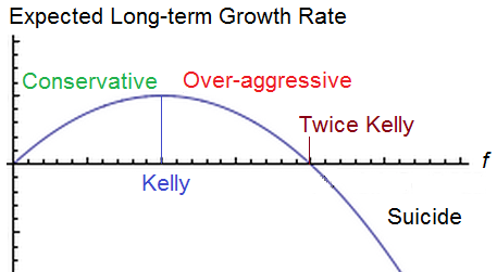
My previous paradigm was guided by this understanding of the relationship of risk:

Unfortunately, every model has certain “assumptions” it must make to construct any particular generalized “model”. It is usually not the model itself you should test, but the assumptions within the model, as well as your own personal assumptions which can only be done by data first. After adjusting and testing these assumptions and thinking more dynamically I can see that this is simply not practical as you will also see in a bit.

At first I had a simulator created to calculate all possible permutations of theoretical trades, but realized the simulator could be improved. Rather than continuing down the direction I was headed, I “flip-flopped” again, instead opting for constant improvement. I instead came up with a spreadsheet that uses the random number generator and a “Monte Carlo simulator” plugin that I view as much more efficient and flexible in terms of the duration of trades in which I want to test. Although it lacks the same degree of precision, it is a productive tradeoff as you can still increase precision in exchange for a more timely monte carlo simulation (with more random iterations).

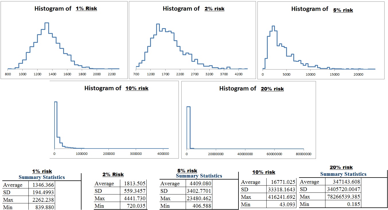
I used the spreadsheet to look at returns dynamically over a finite amount of time such as 300 trades. Out of a thousand traders for example, some percentage may gain 20% while another percentage gains 100% and another percentage loses 50%. Using this data, A histogram plotting all simulated results of each of the thousand random iterations of 300 trades was made for various levels of risk given a particular system. The simulation allows for a change of any one of these inputs (probability of 5 different “results” of the trade, the ROI given each of these 5 “results” the number of traders randomly selected and the number of trades they make). You can even look through random equity curves across all 300 trades at a given risk factor and refresh it with a push of a button to pull up another random trader to get a better sense of drawdown within different points of the system over the course of those 300 trades.

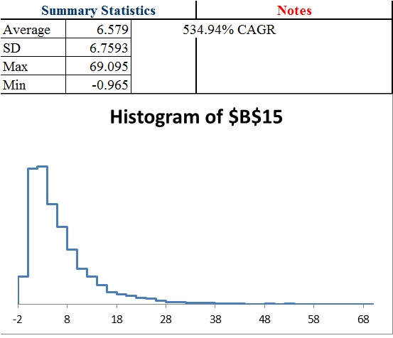
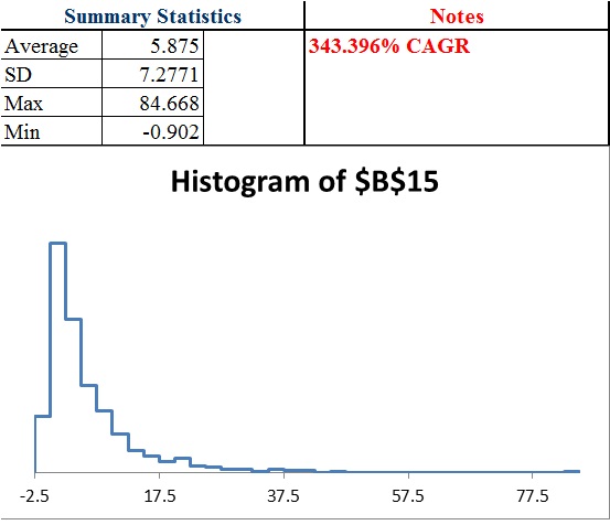
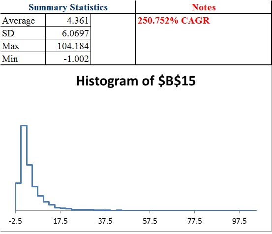
Without further ado, here are some results!

 

pX=probability of event X.

wX=win % (ROI) given event X.

System: p1-5=20% W1=150% W2=50% w3=0% w4=-50% w5=-100% A winning system is presented.

Risk defined as capital at risk since this is an option strategy and you can lose the entire premium.

“optimal F % / full kelly = 14% risk”

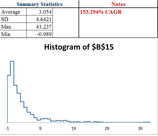
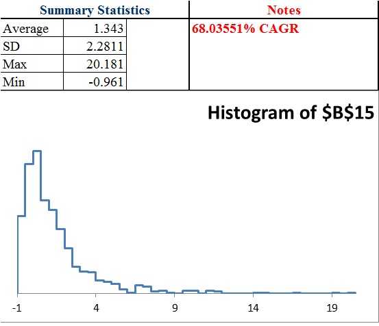
Note the severe skew right. This means as you increase risk extreme outliers begin to skew the average higher than what is “typical”. Skew right means the mean (average) is way higher than the median (average). The “worst case scenario” grows with risk. The probability that you end with a lower than average result (that is not a typo) increases as risk increases risk given a finite amount of time. Eventually the probability of a poor result is so great that as you increase risk the long term geometric return suffers. If you are a true cowboy looking to become an “outlier” and willing to put in the risk, then perhaps that is okay with you, but just know that going beyond the “optimal” amount is destructive as you approach “an infinite number of trades”. Just know the type of CRAZY account volatility you will have to endure, and a large probability that you actually will end down even after 300 trades. That’s almost 6 years at 1 trade a week!

Since I took the time to create this spreadsheet, I can simulate thousands, or if I like, tens of thousands of traders trading anywhere from 1 to 300 trades (or more if I take 5 minutes to set up more) with a given system with a push of the button. I can instantly adjust the expectations of the trading system and see how the results change.

In the next post Titled “Equity Curve of Risk – How Risk Influences Expectations” I show some example equity curve of a particular risk percentages.

 

Comments »

I’ve decided to keep this blog on ibankcoin specific to trends. To keep this blog on topic I made a post at stocktradinginvestments.com titled Kelly Criterion Shows Decreased Correlation Increase Return. The short version is the picture worth a thousand words.

Reducing correlation (and thus increasing your independence of your bets) is important because you can reduce your draw-down, or increase leverage in multiple uncorrelated names and keep the same draw-down with higher long term returns. If you lose 20% you need 25% gain to make up for it, but if you are invested in uncorrelated assets, a 20% loss will be much smaller as your overall portfolio, even if you have multiple uncorrelated bets with leverage. That is the idea.

What’s this all have to do with trend following?

As great as it would be to go “all in” in the best possible area and get every single call right, that isn’t realistic.
This is why I propose you set minimum holdings for risk on assets (stocks,natural resources&commodities,etc) and minimum for risk off assets (currencies&cash, bonds,). But also consider other lowly correlated opportunities. Depending on the trend, you would adjust your weightings, but not necessarily neglect opportunities if it keeps your portfolio’s correlation low.

When stocks go down when you expect them to go up, if you are 100% invested in stocks you not only are down in your position, but you also lose in opportunity to rebalance at lower prices, and in some extremes even change your allocation to be more aggressive. There is a fine balance between trend following and value investing. Value investing principals would suggest that if you are bullish if a stock is at $100 you should be more bullish if a stock is at $90. Trend following is often, but not always, in conflict with this, especially in individual names vs indices. This means you have to be positioned within a trend both to take advantage of the directional move, and also to take advantage of fluctuations in prices away from the trend (contra-trend moves), and to position more heavily if the signals are stronger. But unless you are 100% certain or the move severely outweighs the downside of it going against you, you do not want to be 100% in any asset class. Additionally because daily and weekly volatility (noise) exists within a monthly trend, it still may be right to have some funds you can transfer, despite also being “right” about trend direction since we still may have opportunities to add stocks lower in a monthly uptrend, or add to TLT or “risk off” trade at a lower price in a monthly downtrend (downtrend in equities, that is). For this reason we set parameters.

So we set parameters of maybe 75% maximum and 25% minimum for both risk off (bonds) and risk on (stocks). (You could certainly go with less or more depending on how you want to push your risk, and maybe make an exception or two). We also want to keep what we learned from the linked to post in mind and make sure an area of low correlation has it’s place.) Having this much is a bit more for longer term traders and contrarians looking to preserve enough cash in the event of a big plunge. If you are more nimble and more accurate go ahead and change this, but the rare times you get caught long in a big decline or vise versa, you will often make up for all the opportunity you missed out prior to the big run. Another solution would be to find more pair trades and hedged positions.

Overall though, you have to not only keep track of the trends in stocks, but in the alternative investments.

To keep things relatively simple, I came up with a general guideline to follow for stocks. I started with defining what type of trend we are in . We can be in 4 trending conditions:

Monthly trend up, weekly trend up

Monthly trend up, weekly trend down

Monthly trend down, weekly trend up

Monthly trend down, weekly trend down

Then I threw in overbought and oversold conditions. Within each of those trending conditions there are 4 possibilities. Either no extremes, weekly extremes, monthly extremes, or both weekly and monthly extremes. This gives us 16 potential scenarios to account for. (In reality there are more because 3/4ths of the trend signals for example can signal an uptrend) If you want to use The PPT OB and OS signals there are 32 potential scenarios.

The simple way is rather than make 16 more adjustments, to just note the 16 conditions first then as a rule of thumb subtract 10% from stocks and add 10% to bonds when PPT OB and -1% from stocks and +1% to bonds every additional 0.1 OB points it gets. And for PPT OS to add 10% to stocks and subtract 10% from bonds and add +1% to stocks -1% to bonds every additional 0.1 OS it gets. A more complicated solution would more aggressively sell the overbought signals and more cautiously buy the oversold signals when weekly trend is down (but not oversold), and more aggressively buy the overbought and more cautiously sell the oversold when weekly trend is up (but not overbought).

Then I went through each condition and came up with a potential allocation. To keep it less complicated I just chose “Arbitrage” as the low correlation play mixed in with “treasury bonds” and “stocks”. In reality, “gold” “natural resources” should be considered for “risk on” plays as well. And “currency”should be added in addition to “bonds” for “risk off” plays. Adding in MORE lowly correlated assets and using leverage when appropriate will increase return without at the expense of volatility and long term growth.

In some conditions, leverage is allowed to be added depending upon the asset class.

Since originally writing this article, I decided to keep an eye on these as a guideline, but to change the individual assets. So the principals remains in tact of what percent is “risk off” asset and what percent is “risk on” and what percentage is “arbitrage” or “minimal correlation” to the rest of the portfolio. But the actual percentages changes based on trend.

As you saw in my most recent post the trend trader, I came up with a sort of “model portfolio” to follow in the current conditions. In reality, I may shift a lot more heavily to arbitrage if the deal is right and I may leverage it if the deal itself does not seem to require leverage. For example, if Apple or Google bought something smaller, they would probably have enough cash on their balance sheets and the concern of the deal going through would not depend on availability of credit. If the economy turns south in a hurry as it is vulnerable to do in a monthly downtrend and weekly downtrend, or monthly downtrend with a weekly overbought condition, deals can fall through, so avoiding leverage, keeping that percentage of your portfolio towards arbitrage small, and being cautious makes a lot of sense. There are those I know who just trade pre earnings both long and short certain names, This would be a pretty low correlation type of trade so “arbitrage” when market isn’t vulnerable to sudden credit contraction and rising LIBOR rates isn’t the only way to have a near 0 correlation, it’s just the one I am going with. Earnings has larger moves in a short period of time and may require greater number of trades at a smaller position size to reduce potential for a large downside swing in portfolio size. What I am trying to communicate here are the PRINCIPALS though…

You can use the trends, or use value weighting or whatever signal you want for adding lower and selling higher via rebalancing, or more aggressively repositioning your allocations. But A very often overlooked goal is how your overall return on risk within a portfolio comes out. And to do that, it requires multiple assets with low correlation weighted towards which ones have a higher probability of equal upside/downside or greater overall edge, and a focus on low correlation. Once you can accomplish that, you can determine your return based upon leverage and how aggressively you position one way or another.

I have another post I will work on that further illustrates this difference in leveraging up your returns vs no leverage given everything else is roughly the same.

Comments »