Ever wondered how increasing the number of trades in a period changes your performance? I’m really close to figuring that out to a very specifically defined calculation. The one missing variable is “correlation”. I don’t know how to account for it and how correlation impacts probability.
So for this experiment we’re going to assume binary outcomes of -100% or +250%. I’m going to assume my own variation of the kelly criterion strategy so I can model them at an equal amount of risk(?).
The logic is: If the maximum you can bet to maximize geometric growth at one single bet is 10%, then after a single bet you are left with 90% of cash. If you lose, you will be making a bet that is 9% of your initial capital anyways, so we can allocate 19% for two trades that we hold simultaneously provided there is zero correlation. If we are going to make a 3rd trade we are 81% cash so we can add an additional 8.1% risk and divide the total amount at risk by 3 and so on. It’s possible you can risk slightly more than 19% for 2 but less than 20% because a loss isn’t guarenteed. We will position as if the first position lost due to the possibility of it losing and the nature of overbetting providing less return at increased risk (where as underbetting provides less risk and return only declines slightly)
Background
For some brief background on how the risk amount to maximize growth, see the Kelly criterion. Essentially you are going to take (O1^N1)*(o2^N2) where O1 is the wealth multiplying outcome at the given position size, and N1 is the number of times you produce that outcome. For instance, at 1% position size with 250% gain and 100% loss for outcomes, O1 is 1.025 because a 1% position producing a 250% gain multiplies our wealth by 2.5% or a factor of 1.025.
This is calculated by
1+(.01*2.5)=1.025
And the loss is .99 which is calculated by
1+(.01*-1)=.99.
So for 20 wins and 30 losses the equation for how much our wealth changes is (1.025^20)(.99^30).
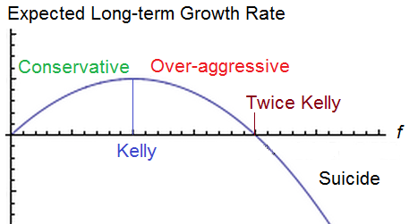
The Kelly criterion reverse engineers the position size to solve for the position size which maximizes geometric rate of return based upon your assumptions over an infinite number of bets. As volatility increases, eventually return decreases. The kelly bet seeks the point at which you can no longer improve the return without much respect for the volatility. In reality, you’d probably wish to respect a fractional kelly strategy if you want to reduce risk. It’s a good way to compare systems at an equal amount of risk. Right now I’m using a modified kelly. It is similar logic as the kelly but not the kelly exactly to increase position size based upon multiple held positions.
You could manually adjust the position size for very large outcomes with a proportional amount of wins and losses until you can’t seem to increase it to approximate the solution, or just use a kelly criterion calculator. You can run more complex calculation with more than 2 outcomes, but for now I’m just using 2.
Optimal Bet Size
So the optimal bet size for a single bet is 9% given 35% chance of a 2.5 to 1 payout.
We can then solve for the optimal bet size for 40 bets assuming zero correlation between trades but with 40 trades held during the same exact time period. There’s an important distinction here. Rather than multiplying our wealth by 1.025 with each win, at this point we are only adding 0.025 to the total portfolio per win because we don’t get the benefits of compounding when the trade is placed. Similarly, if we hold 40 1% positions at once and lose them all, we don’t lose 1-(.99^40)=.331 or 33.1% but instead lose the full 40%. So the first formula is not sufficient in describing what happens to our wealth. This is also where correlation is a bigger liability than the formula currently realizes as the chance of greater drawdowns increases as the correlation increases.
As explained before, we are going to assume a full kelly and then an additional full kelly of risk with the remaining capital for each additional bet. Since the full kelly is 9%, that means the cash on hand remaining is .91 of our portfolio which can be multiplied for each of 40 bets to determine how much cash on hand to keep
or .91^40 to equal 2.3% which leaves 97.7% at risk divided by 40 is 2.4425% per bet.
We can repeat this for 30 bets, 20 bets, 10 bets and 5 bets to construct a table of optimal bet sizes per bet.
Bet size given total number of positions.
| 50 bets | 1.98209% per bet |
| 40 bets | 2.44251% per bet |
| 30 bets | 3.13649% per bet |
| 20 bets | 4.241775% per bet |
| 10 bets | 6.105839% per bet |
| 5 bets | 7.519357% per bet |
| 1 bet | 8.9999999% per bet |
Now we can construct a simulator that sums the total % gained per bet over a period for 12 periods and randomizes the outcome according to the probability.
Excel gives us a function =RAND() which delivers a number between 0 and 1. If that number is less than .35 it will deliver a 2.5 times the position size outcome. If it’s more than .35 it will deliver -1 times the position size as the outcome. All position sizes for a period will be summed up and the number 1 will be added and then multiplied to the portfolio size and then the fees for the period will be subtracted. 12 periods will be simulated giving us a yearly total. We can then run through 1,000 different yearly results and see the distribution of results, the average, and even estimate the compound annual rate of return
This way we can see when the benefits of diversification outweigh the costs for smaller 5 figure portfolios where fees eat into profits. I am probably over estimating fees slightly as I used $6 per trade and assumed buys and sells for all trades, where in reality there is only an opening trade for 100% loss trades.
The CAGR is a crude estimate as the simulator only gives me the first 100 results. I am basically taking the returns plus 1 and multiplying them all and estimating X where X^100 equals 1 minus the multiple factor of the first 100 results. The CAGR will be substantially less than the mean outcome. TO illustrate imagine a 25% average return where the results are -50% of your portfolio and then +100% The actual CAGR of an equal amount of -50% returns as 100% returns would be zero, not 25%. The CAGR reflects the loss due to volatility.
I assumed a 20,000 starting portfolio and $6 fees with the assumption that there was both a buy and a sell order for each trade. Trade fees were deducted after each period’s multiplier was applied.
40 trades @ 2.4425% position per bet
30 trades @ 3.1365% position per bet
20 trades @ 4.2418% position per bet
15 trades @ 5.0466% position per bet
10 trades @ 6.1058% position per bet
5 trades @ 7.5194% position per bet
1 trade @ 9% per bet
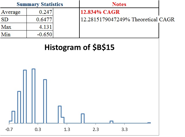
For 12 independent trades or 1 per 1 month period, the theoretical gain is .97% growth per bet or 1.0097^12=~12.28% growth per year… theoretically. But that’s over the time horizon of infinity and as you can see by the distribution should 1,000 traders have the same exact expectation, the actual results over a year can vary wildly. Also, with only a $20,000 account taking too much risk or not enough can result in problems should losses occur early because of the size of trading fees being a flat amount.
We find we can greatly enhance the return by adding more position sizes, but the benefit of diversification decline with each additional bet.
Adjusting For Correlation
While I think the above can give you good idea for how many trades for a given portfolio size you should hold at once (and we could easily adjust the calculation for half of the initial kelly bet), we still have yet to develop a system that adjusts bet size based upon correlation. What I believe is true is that as correlation approaches one, the total amount risked should approach the single kelly bet. Afterall, if you bet all your capital on multiple trades of the same coinflip, it would be no different than betting a single bet on that coinflip. In other words in our previous example as the correlation increases the total amount at risk should approach 9%. This means that the ideal bet in reality is somewhere between the bet size calculated above at the correlation at zero (that has been calculated as shown in the prior table) and the correlation of 1 which is 9% divided by the number of bets.
For instance, if the correlation was 0.50 across 20 bets.
A correlation of zero suggests [1-(.91^20)]/20=4.241775% per bet.
A correlation of 1 suggests 9%/20=.0045 or 0.45%
Since the correlation of 0.50 is the midpoint between 0 and 1 we can average the 2 and get 2.35%*
*but that’s only an approximation.
Unfortunately the relationship may not be linear, so while we can be sure the optimal bet size for maximizing CAGR across 20 simultaneously held bets is somewhere between 0.45% and 4.241775%, we can’t be sure it is the exact average of 0.0234589 or ~2.35% per bet.
I also want to look at “half kelly” strategies in 2 different ways. One is dividing the per trade bet by 2. So for 40 bets if we calculated 2.44% the half kelly could be 1.22% per trade. That halfs the total amount of capital at risk. The other is using a 4.5% number initially, and so a 0.955^40=~15.85% cash on hand or ~84.15% invested divided by 40 or 2.10365% per trade instead of 2.44%. We can see that that is still much more aggressive than halving the amount per bet.
Normally the half kelly solution provides 3/4ths the return at 50% of the volatility of the full kelly. This is really promising for multiple bets when we can reduce the amount at risked by only a small amount and still be at an equivilent of a half kelly strategy in some regards.
In the future I also want to come up with a different calculation such as solving for the “probability of a 50% decline or more in a year” (or probability of 100% gain for example). This is pretty easy to set up.
If the result is -50% or less in a year, a simple formula will give me a 1. Otherwise zero. The average is the probability of this event. This helps you better model the probability of achieving a certain result (such as 100% return) while measuring it against a probability of a negative outcome (such as 50% loss) so you have a different way to compare risk and reward of position size and number of trades and understand expectations.
For now it seems more bets is better up to a certain point where the quality of opportunities and expectations as well as the fees become problematic. It’s hard to identify where that is, even with thousands of simulations because of the increased “skew” (the expectations become increasingly dependent upon a smaller and smaller probability of a more and more spectacular outcome) as risk and number of trades increases. Also, as your bet size decreases the aggressiveness and increases the amount of trades, the fees should become more problematic which I think we will see in a half kelly and 1/4th kelly simulation. Lowering your position below 0.50% when you have a $20,000 portfolio for example might become a problem and eat into returns too much. As such as we seek to decrease our risk, we will eventually have to decrease our number of trades or else position size will be too small given the fees to provide as big of an edge.
If you enjoy the content at iBankCoin, please follow us on Twitter


Hattery that’s quite an analysis, thanks for sharing it. Pardon me if you covered this, one comment- Something I found fascinating about simulators- for a given set of parameters different runs of the same period produced different results. If this is not an error in the simulator I used, it is interesting considering snapshots of a never ending series of trades.
If I understand correctly, yes, the design of this simulator in particular is to use a random number generator to produce a return consistent with the 35% probability of 250% gain and 65% probability of -100% on invested capital for a given position size for each trade. It pulls a random number between 0 and 1. If the random number is less than .35 then the 250% gain occurs, otherwise a 100% loss in the given position size. The period of say 40 trades represents a month and so the simulator produces the result of 12 periods for one result. The Monte Carlo simulation is run to update all random numbers and automatically record the outcome 1,000 or 5,000 times and Graphs all outcomes. You can also use math to determine what the outcome would be exactly in more specific situations, but the simulator better captures the range of possibilities and how likely an outcome is.
The position size has a very significant impact on the results… but the number of trades or “bet” the cost of fees, and the correlation all play a role in the total amount of capital you can have at risk as well as the position size. These are all tremendously important variables in determining how much money you have made at the end of the year.
This is pretty heavy analysis considering human trading is more judgement and discipline over optimization. It is good for people to see what people like #yolowolf do wrong in trading by crapping out before they find consistency. Maybe you and Raul could open an hft algo shop though.
Judgement and discipline are absolutely important and I’m glad you pointed that out.
The point is to try to at least get people to see the big picture of what defines good judgement when it comes to position size and how to know where to establish the line to be disciplined in not crossing. Maybe my examples are overly specific, but I did this to establish an apples to apples comparison of risk at maximum growth. Risking any more for a set number of positions would reduce return.
People like YOLOWOLF are a dime a dozen, but few of them give people a chance to watch the blow up happen.
Perhaps it was lost in translation of all the jargon and I failed to really emphasize the point. The methods I used could also be applied to a different system if someone was looking to optimize their particular system. But I did not optimize to say here’s a system to apply or here’s a method to optimize. Rather, I did it to illustrate principals.
The biggest illustration that I discovered from this work is this:
1 trade ~12.8% return
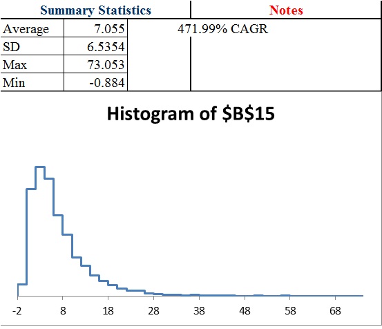
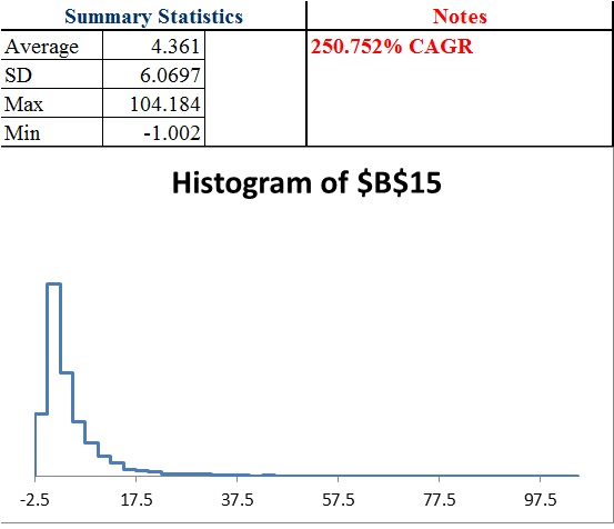
30 trades: >500% return.
That’s a big difference and shows how increasing position and reducing correlation can work together (provided you maintain an edge) in boosting return.
An inference from this:
Given 30 trades are made, as the correlation approaches 1, the return would approach 12.8% (less due to more trades requiring more fees), and as the correlation approaches zero, the return would approach >500%…
That is only true at an maximally aggressive bet size adjusted for correlation, but for a fixed bet of out of the money options of 2% position size, returns would still improve up to say something like 45 positions and the optimal amount of bets would decrease as correlation increased.
The exact numbers are not important. I could come up with totally different expectations at a different account size and more trades at lower correlation would still be better (to a certain point where fees, correlation and diminishing opportunities would hurt performance).
Reducing correlation and position size are probably far more important than many people realize in determining returns and drawdown size. It isn’t everything and you still have to actually have an edge (which is where trading skills, discipline and judgement come into place).
It’s striking how individual trades with favorable odds can yield a long-term loss simply due to an excessive position size.
Optimizing the size of simultaneous independent bets would seem to require considering all outcome combinations. In the case of identical odds per bet, a binomial expansion can apply.
Using the example with -100% or +250% with a 35% chance, where the optimal size for one bet is 9%, solving for five simultaneous bets using a binomial expansion to maximize the expected log return (geometric growth) yields about 8.421455055% per bet. That said, so many terms could easily yield an error here due to a simple typo. And this example doesn’t even include correlation.
Thanks for the article Hattery. It spurs further investigation.
Glad you learned something and that I inspired you. It sounds like you have a good head on your shoulders on some of the technical aspects of this and it seems a better grasp on the mathematics than I do and looks like you know where to go with it.
Yes, being able to lose over time despite having a positive edge certainly flies in the face of an “expected value” mindset and conventionally taught ideas on risk, but there are certainly limits to risk. Lack of certainty of your edge is another thing you could try to model where the return is more randomly selected between 200% and 300% or 30% and 40% for example (or applying a standard deviation to your expectations)
I’ll have to look into binomial expansion. The term sounds vaguely familiar but I kind of learn as I go with most things. I know that the idea behind the Kelly criterion is to maximize the expected logarithmic return, so if binomial expansion can help you solve that, it’s probably more accurate. I took the shortcut of investing as if each prior Kelly bet was lost, then dividing the at risk capital by the number of trades. In reality, accounting for the possibility that it could also gain probably should allow for slightly more risk which explains why I had a lower amount.