This is an ongoing series on how to construct and implement a position sizing spreadsheet to help you optimize the money management aspect of your strategy. It will be capable of helping you maximize things such as probability of reaching a certain return in a year, or probability of reaching a certain percentage return or capital amount by a certain deadline, or minimizing your chances of ending up down a certain amount over X trades. This will help you to trade more consistent with your goals and come up with more realistic expectations.
Part 1 WoodShedder Time! Creating A Quantifiable Approach To Position Sizing
Part 2 Building A “Position System Simulator”
Part 3 Building Cover Sheet, Determining Probability of Results (Position Size Simulator Part 2)
Part 4 Adding To The Cover Sheet
Part 5: Setting Up The Calculations
As stated in the past, I want to create a spreadsheet that simulates all possible combinations of results with a given “weight” according to the probability of each result happening.
Formulas are the “engine” behind this spreadsheet. If you want to know the probability of a 20% drawdown over a series of 5 trades or 25 trades, or the probability of any result over X trades… you have to have formulas that can calculate that, given certain data.
The cover sheet gives us a “starting bankroll” and % of capital used per trade and the data that we can set up. We want to use this data plus the data for the “fees” in the cover sheet and the ROI on the calculation sheet to determine the result of a set of 5 trades and repeat for each possible combination of 5 trades. We will start with 1 single trade.
To set up this formula to solve for all, we must use the cover sheet. Lets come up with the formula AFTER fees for trade 1.
(Starting Bankroll * bet size*ROI of trade 1)=return in dollar amount after one trade before fees
+ Bankroll= bankroll in dollar amount after one trade before fees.
– ((# of contracts*fee per contract)+Commission per trade) = bankroll after 1 trade (fees included).
We can clean this up a little and simplify this to:
Bankroll after 1 trade=(Starting CAPITAL towards trade * ROI1)+Bankroll – (fees).
We just need to run the calculation on the cover sheet for FEES and “Starting Capital towards trade”. This will require less switching back and forth between tabs and make the what formula is accomplishing once we run it on the spreadsheet less confusing.
Now trade 2. We will be left with a different amount of capital from trade 1, and use a different bet size in dollar amount. So now we must use the formula:
$ at risk * ROI + Bankroll – Fees
But $ at risk depends on CURRENT bankroll times bet size and CURRENT bankroll is based upon what we just calculated. Additionally FEES depends upon # of contracts which depends on current bet size.
so $ at risk is replaced by
(previous bankroll * bet size % )
And Fees is replaced with
((# of contracts) * (fee per contract))+ commission
(# of contracts) is then replaced with
(Current Bankroll * bet size %)/option price (we won’t round and will assume fractional contracts. In real life your bet size and results will vary as a result depending on how you choose to round).
The complete formula is thus
Bankroll after trade 2=(Previous Bankroll * bet size) * ROI + Bankroll – ((((Current Bankroll * bet size %)/option price)*(fee per contract)) + commission)
Bankroll after trade 3,4,5 is actually the same so we can replace the 2 with X.
The 3rd, 4th, and 5th trade is simply the same formula, only adjusting “current bankroll” to reflect the results of the bankroll after the previous and most recent trade.
So now we simply convert it into “excel language” we want to substitute each aspect of the formula with the corresponding cell on the sheet or on the cover sheet that corresponds with that particular data set.
Then we will want to use an easy feature to make sure that formula is applied in a similar manner for ALL relevant cells, rather than just one.
Setting up the formulas:
What may make things easier, is if you just copy and paste the formula in it’s current form, and then use a find and replace function to replace the text “Previous Bankroll ” by “N3” or whatever corresponds to the cell which contains the bankroll after the completion of the first trade. Or in the case of the first formula for the first trade, replace “Starting Bankroll” with “cover!C19”. There is one problem with that as the “previous bankroll” for each row of cells will be different, as they will correspond to different potential ROIs. We will get to adjusting for this in a bit so you can apply the formula to all cells For now I am just going to list the formula according to the way I have set up the spreadsheet.
Bankroll after 1 trade=(Starting CAPITAL towards trade * ROI1)+Bankroll – (fees)
Translates into the excel notation:
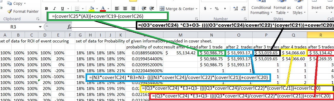
=(cover!C25*A3)+cover!C19-(cover!C26)
The only variable you will want changing for the entire column (in this case the “N” column), is A3. For row 3 it’s A3, for row 4 it’s A4, etc. A3 corresponds to the ROI for that set of trades and this will occasionally be different.
The formula for the remaining trades are
Bankroll after trade X=(Previous Bankroll * bet size) * ROI + Bankroll – ((((Current Bankroll * bet size %)/option price)*(fee per contract)) + commission)
That translates into trade 2 cell has formula
=(N3*cover!C24) *B3+N3- ((((N3*cover!C24)/cover!C22)*(cover!C21))+cover!C20)
trade 3
=(O3*cover!C24) *C3+O3- ((((O3*cover!C24)/cover!C22)*(cover!C21))+cover!C20)
Trade 4
=(P3*cover!C24) *D3+P3- ((((P3*cover!C24)/cover!C22)*(cover!C21))+cover!C20)
Trade 5
=(Q3*cover!C24) *E3+Q3- ((((Q3*cover!C24)/cover!C22)*(cover!C21))+cover!C20)
Illustration with all formulas included for people that are more visual (every formulas added in over image for clarification).
That gives us the outcome after 5 trades given ONE single set of 5 trade combinations. There are over 3,000. There is no way we will do this all manually.
Now, the only thing that really changes as we set the formulas up for all possible trades is the number after A for trade 1, numbers after N and B for trade 2, numbers after O and C for trade 3, P and D for trade 4 and Q and E for trade 5. The numbers must change to correspond to the row where as everything else will remain the same.
If you click and drag the formula, it changes ALL numbers, rather than just the ones you want.
There probably is an easier way than the way I will suggest, so if anyone is an excel guru and knows it, I would like to hear it, but this is what I do…
Set up a separate sheet that basically isolates the component of the formula that you want to change from the one’s you want to keep the same. Keep the equal sign separate so it doesn’t try to calculate anything or autoadjust the formulas.
In the first trade we only need to adjust 1 number after A. So copy each column and hit CTRL+SHIFT+Down Arrow to select all and then CTRL+V to paste. For the next column you can just double click on the bottom right hand corner of the cell to autocopy and paste all the way down until the last row that was used. However, the column you want to modify you must adjust the formula first. In this case, we want each formula to contain 1 number larger than the previous so we use the formula =C2+1 and excel will run that formula for all cells down the entire column.
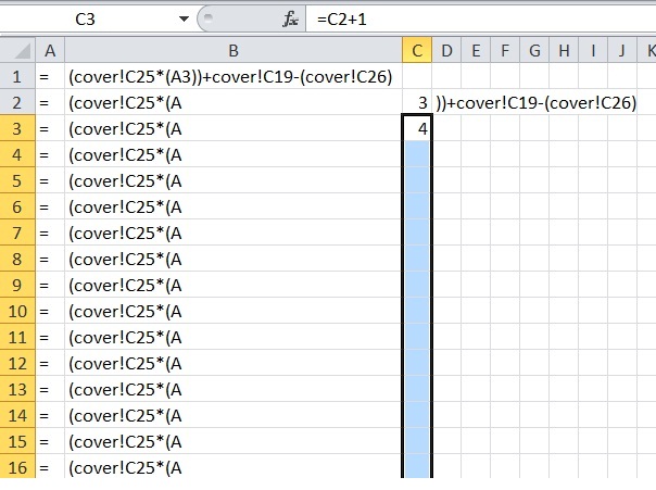
It will do this and then eventually fill in with numbers.
Now we have to bring the formula back together so we can paste it back into excel on the tab we want to. So we need to copy and paste all the formulas we want to use into a notepad (so page down and highlight about 3200 rows or more and then use CTRL+C to copy, and open a notepad then press CTRL+V to paste)
The issue at this point is that between those cells it automatically created a “tab” over or a separation between the formulas, so highlight the spaces and copy them and do a find and replace to replace the spaces with… nothing(leave the replace blank).
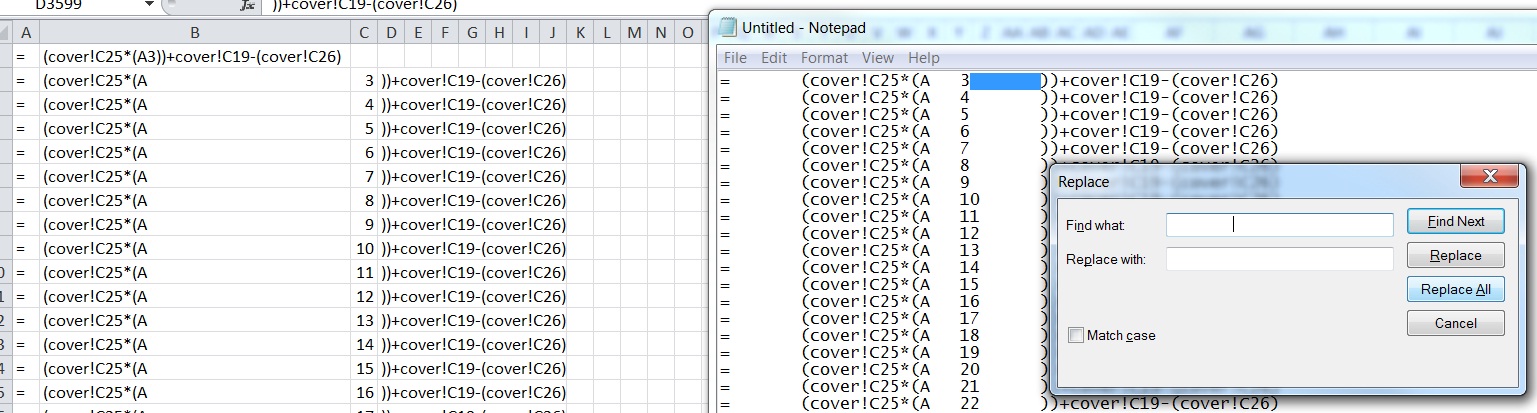
Replace all!
Then copy and paste this BACK into the excel spreadsheet so you can put in all the formulas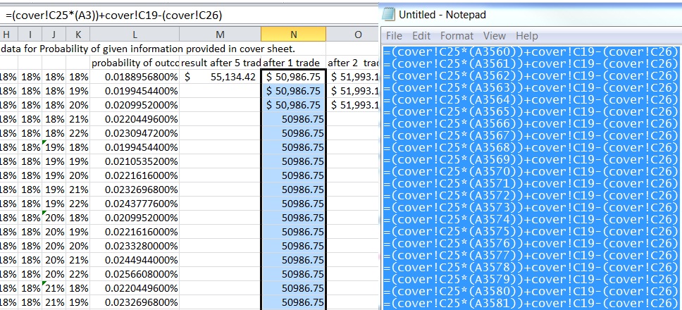
Repeat for all rows. The easy thing is, the find and replace for after trade 2 and after trade 3 is incredibly similar. You can simply change a couple letters in each formula on the sheet and double click the corner box to copy and paste down the row rather than re enter in the entire formula and isolating each component after setting it up for row 2 and 3 and 4 and 5. One bit of advice, separate the equals sign, plus sign and minus sign in it’s own cell, otherwise it will try to run a formula and change it to contain an equal sign.
This should only take about 5 minutes to get all of the formulas set up in this manner.
—
Now what do we have? We have the RESULT after 5 trades for every possible trade, and we have the probabilities of each event occurring. We are real close to finishing this up.
We will wrap it up by a few post that sets up a formula to weight each event by a probability of occurrence and adding a weighted average and then using a formula, apply this and expanding it to 125 trades, rather than just 5 and our work will be mostly complete. I may add a “bonus” section of this series to clean up the data and give us conclusions right on the cover sheet automatically and other features that may be useful to add. I would like to adjust this to come up with a spreadsheet that allows you to consider making multiple trades, rather than just one if I can figure out how.
But as mentioned previously, at some point I want to get into discussing my philosophy as well, and converting that to a dynamic strategy, which is currently in development.
If you enjoy the content at iBankCoin, please follow us on Twitter