Insignia Brand BlueRay/DVD Home Theatre System SUCKS

I went to Best Buy today and purchased an Insignia model NS-BRHTIB Blue-Ray Disc Player and Home Theatre System. It was on sale, and the audio sounded good in the store. I have been operating with a 5 year old DVD player and awful sounding AKAI home theatre system, so it was time to upgrade.

So what is the problem?

After tearing down my old system, and setting up the new system, which took a couple of hours, THE SON OF A %@#$! DOES NOT WORK.

To be clear, I can access the menu on the Insignia, adjust settings, etc., and my HD TV recognizes the Insignia via the HDMI input, but when I press play, I get audio, and no video.

I went to the Insignia website, downloaded the firmware, and updated the disc player. It didn’t make any difference.

I then called Insignia customer support. While they were very friendly, in less than 5 minutes, they had determined that I should just take it back to Best Buy and exchange it for another Insignia product, or get my money back. Clearly, this is a known issue with this model. In fact, on Insignia’s own site, there are several reports in February of this problem with this model. Insignia’s solution? Take it back.

So I’m about to spend another couple hours breaking this SON OF A #$%@! down and putting it back in the box to take back to Best Buy tomorrow. I’ll have about 6 hours total involvement in trying to get this piece of crap to work.

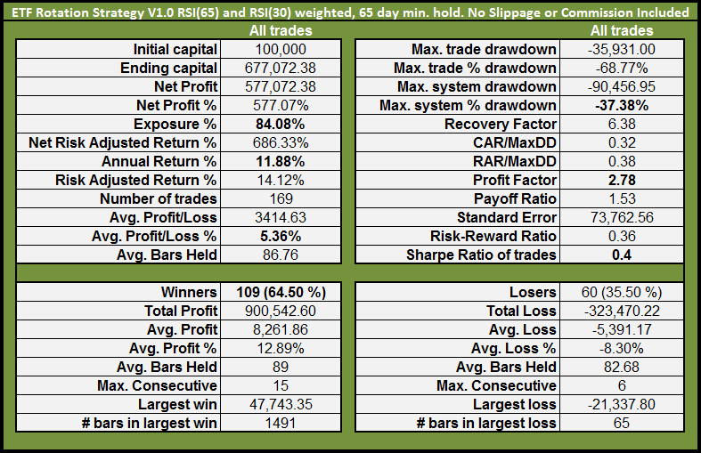
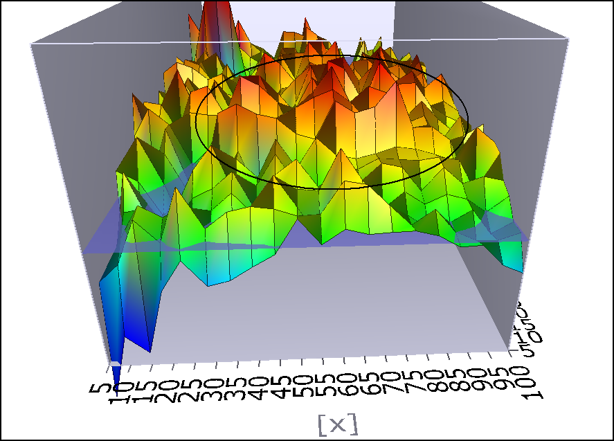
Please forgive me for not posting another installment tonight on the ETF Rotational System. I’ve wasted my blogging/researching time on this PIECE OF CRAP INSIGNIA product.

Comments »

I’ve taken a short break from the ETF Rotational Strategy series to try and figure out what is going on with this recent pullback. To be clear, I want to short this market. (In fact I did, this morning). It seems I’m not the only one, as even our dear Blogfather is sitting on mounds of cash, waiting for a lower entry for deployment.

After today’s finish, which “looks” bearish to me, I decided to run yet another study to see if there has been any edge to getting short here. I just wanted to check my head, as revenge trading and acting on emotional whims is no way to beat the market.You might recall the previous study did not paint a bearish picture. Still, today’s setup is the gloriously bearish Honey Hole pattern, which iBC old timers might remember served us well back in 2007 and 2008.

In case you were not able to avail yourself of iBC wisdom back in tha day, the Honey Hole pattern comes after an index has fallen beneath the 50 day moving average, and then rises beneath it, testing it, preferably following a multi-day run. It also helps to have RSI(2) rising above 90.

In the chart above, there are other indicators that are not so bearish, such as the recent MACD cross, and the recent peak in ATR(10). In regards to ATR(10), volatility tends to peak near bottoms, and it appears it might have peak already, near the bottom of the pullback.

Anyway, let’s test this honey hole.

The Rules:

1. 3 previous days all had closes higher than the opens.

2. Today, the close is less than the open.

3. The close is less than the 50 day moving average.

Sell short the SPY at next open and cover the short N days later. No commissions or slippage. There were 53 instances of this setup over all SPY history.

The Results:

Alas, it appears that there is not much honey in this hole, unless we are willing to wait around for over 2 months. Even the percentage of winning trades (axis on right side) is dismal, showing a greater chance of losing than winning.

As the proud borrower of [[SSO]] , based on these tests, I will be looking to cover this position quickly, on any weakness. While it is probable that some weakness can be expected over the next few days, the edge is not near strong enough for me to stay short with any real conviction.

It seems that the bears are early here at the honey hole. The conviction trade remains on the long side, deploying any cash into near-term weakness.

Comments »

Many of the broader market ETFs have recently seen their 20 day moving averages fall and cross beneath their 50 day moving averages.

Is this is good time to get short?

The Rules:

1. The close is higher than the 200 day moving average (ensures there is still a primary up-trend).

2. The 20dma crosses beneath the 50dma.

3. Sell short SPY, IWM, QQQ on the next open.

4. Buy to Cover n days later.

No commission or slippage included in tests.

The Results: Average Trade

The Results: Percentage of Winners

Summary:

With the possible exception of [[IWM]] , it appears that there has been no edge in getting short after the 20 day crosses beneath the 50 day average on these three ETFs. In fact, for [[SPY]] and [[QQQQ]] , the setup has been more effective as a buy signal.

Comments »

Read Part 1 and Part 2…

In the comments of Part 2, Jeff Pietsch suggested running the system over the Fidelity Select Fund portfolio used in this series of tests to gain some insight on how the system would perform over a longer time frame. Not a bad idea, and simple to test. Long story short, with every setting, parameter, etc. the same as Part 2 except run over the Fidelity Select Fun portfolio, the system does a CAGR of 12.03%, with a pretty equity curve. It does suffer from drawdowns bigger than I would like, but would easily be improved with the addition of a moving average filter. The FSF portfolio generates its first trade in 1985, and by 1987, the system is fully diversified across four different funds.

The point of all this is was determine if our settings of RSI(65) and a minimum hold time of 65 days, are robust. (Return to Part 1 how these settings were determined). I do not think that I am able to say without a doubt that the settings are robust, but it is safe to say that they work very well using the 40 Fidelity Select Sector funds. I’m not sure why the FSFs tend to work better than ETFs, but my go-to suspicion in these kinds of circumstances is that funds that are priced once a day are not as likely to have the edge traded out of them.

Using 2 RSI Calculations and Weighting them…

In Part 2 I discussed using a technique which uses a longer and a shorter RSI calculation, weighting each differently, and then summing them to create our ETF rank.

I decided to use RSI(65) for our longer length and RSI(30) for our shorter length.

How do we weight them? I used a higher weight for the longer RSI length and a lower weight for the shorter length, so that the calculation looks like this: Rank=(RSI(65)*.6)+(RSI(30)*.4)

I have some thoughts about the weighting process, but I’ll save them for the summary/caveats.

Results with 2 Weighted RSI Calculations

Summary of Results:

Using 2 weighted RSI calculations to rank the top 4 ETFs improves results, doubling the compound annual rate vs. the previous version. All metrics, including maximum system percentage drawdown, have improved versus using a single RSI(65) calculation to rank the ETFs.

Caveats:

If the parabolic equity curve has suggested curve-fitting, then consider yourself astute. Indeed, the .6 and .4 weights are near optimal. It is pure accident that I started with .6 and .4. I was simply looking for a greater weight for the longer RSI length. Using weights of .7 and .8 for the longer length and .2 and .3 for the shorter length result in CAGRs similar to using RSI(65) on its own, but with slightly improved drawdowns.

To gain understanding of the influence of the weights, I ran a walk-forward optimization on the weight parameters, allowing each weight to be anywhere from .1 to 1, adjusting them in increments of .05. The results were very promising and showed that the optimal weighted values consistently maintain their edge long enough into the future that the out-of-sample results are comparable to the in-sample results.

But there was something more interesting about the walk-forward results, and that is that the weights seem to adjust according to the market regime and volatility. While I haven’t thoroughly testing this premise yet, it seems that we need a higher weight for the longer RSI length and a lower weight for the shorter RSI length when the market is demonstrating a medium to low volatility uptrend, while the shorter RSI length needs a stronger weight than the longer length during periods of high volatility. Anyway, in the future, I may try to quantify this so that the weights are switched automatically based on the market regime.

Next, we will take this 2 factor system and add another factor, the moving average filter. We want to determine which is better for mitigating drawdowns: Inverse ETFs in the portfolio, or a moving average filter.

Comments »

Well its time to take a look at how this thing actually performs.

But if you are new to this series, you might want to take a look at Part 1.

To recap:

System Specifics

The system will calculate the momentum/strength of each ETF in the portfolio, and then based on that metric, rank the ETFs. Version V1.0 will use RSI as the proxy for momentum.

• The top 4 highest ranked ETFs will be bought on the next open after the signal to rotate.
• Each ETF will be held for a minimum number of trading days.
• At the end of the minimum hold time, the ETF portfolio will be ranked and re-balanced, with all sells taking place at the close.

Version 1.0 will be using only 2 factors, which are RSI(65) and the minimum number of trading days to hold the ETFs, which is also 65. Again, review Part 1 to see why those inputs were chosen.

The Results:

Summary

SPY has a compound annual rate of 5.34% over the same time period, so V1.0, once commission and slippage is accounted for, has probably not done any better than a buy-and-hold strategy.

Obviously, the system has a propensity for large drawdowns, and that issue must be addressed. That will be an easy fix/test, and not very much fun since it is so easy. Therefore, we’ll make improving V1.0 a little more challenging. What I will do for V1.1 is use two different RSI calculations, weighting both of them differently, and then summing them to get our ETF rank. Any of you who read the comments section here have probably seen Jeff Pietsch of Market Rewind fame mention this method a couple of times. Using two different period settings and weighting them should be more interesting than applying the old moving average filter to deal with the drawdowns, and will keep the system simple 2 factor model, for now.

One other thing to mention is that there were not but a few ETFs trading back in the middle 1990s. Because the system is requiring 4 ETFs, you’ll notice that some of the early trades are held for a few years, because there were simply no other ETFs to rotate in to. This issue disappears after a few years and other ETFs come on board. You can explore all this by viewing the trades, which I’ve linked to below.

View all the trades here: ETF Rotational System V1.0 All Trades

Comments »

It might be hard for technicians not to be bullish after Friday’s (2/5/2010) close.

After a tiny gap-up on the opening, the SPY traded down ~-2% and then reversed to close just above the open and above yesterday’s close. This action creates an interesting candlestick which shows the battle between the bulls and bears. (See circled candlestick on chart).

Another interesting feature of Friday’s trading was the surge in volume. Volume on Friday surged to close more than 2x greater than the 50 day volume moving average. The chart shows the number of shares trading hands was reminiscent of the volume surges when the market was forming the March 2009 lows.

MACD looks as if it might have made a higher low, diverging from price, while VIX closed more than 5% above its 10 day moving average (this VIX setup is a high-probability buy signal if one closes the trade when the VIX closes back beneath its 10 day moving average).

All these appear to be bullish signals.

I have to admit, I was feeling pretty bullish after seeing the market reverse from its death spiral to close higher.

I decided to test a set of conditions similar to the characteristics of Friday’s trading to see what typically happens afterward.

The Setup

Using SPY…

1. One day ago, the market closes at a new 20 day low.

2. Today, the H-L range is greater than 1.5%

3. Today, volume is more than 2x greater than the 50 day moving average of volume.

4. The close is higher than the open.

Buy the SPY next open, and sell the close n bars later.

Results

About the axis of the graph.

• The horizontal axis shows how long the trade was held. Exiting on day zero means the trade was closed the same day it was opened.
• The left vertical axis shows the percentage of winners
• The right vertical axis shows the percentage gain of the average trade.

The setup appears to have a bullish edge.

Caveats

There were only 22 instances of this setup since 1995.

The same conditions as tested above also existed on Friday’s close for IWM, QQQQ, and DIA. The setup is decidedly bearish on the QQQQ and IWM over the full 30 days after buying and only marginally effective for the DIA.

Because the volume surge on Friday was surprisingly large, I increased the surge requirement to 2.5x the average. This adjustment halved the number of instances of this setup to 11, and made the setup only marginally effective up to 5 days after the buy day, and then bearish to neutral for the following 25 days.

Considering these caveats, you may decide, as I have, that the setup may not be as bullish as it first appeared to be.

By the way, if you enjoy reading this type of study, the undisputed master of the genre is Rob Hanna over at Quantifiable Edges.

Also, Michael Arold did some similar research over on his blog, and even posts a chart of each instance of the setup: The Friday Reversal Trade.

Comments »

For history on how we got here…

Thinking About a 4 Factor ETF Rotational System

More Thinking About Factors

Proposed ETF Portfolio for Rotational System

The first runs will test a very basic system as I want to be able to see if adding any more complexity to the system improves it (and how it improves it) in any way over simpler versions.

System Specifics

The system will calculate the momentum/strength of each ETF in the portfolio, and then based on that metric, rank the ETFs. Version V1.0 will use RSI as the proxy for momentum.

• The top 4 highest ranked ETFs will be bought on the next open after the signal to rotate.
• Each ETF will be held for a minimum number of trading days.
• At the end of the minimum hold time, the ETF portfolio will be ranked and re-balanced.

Version 1.0 will be using only 2 factors, which are RSI(x) where x represents the periods, and the minimum number of trading days to hold the ETFs, represented by y.

Lets take a look at how these factors play together, using AmiBroker’s 3D Optimization graph.

The most obvious feature of these graphs is that they are peaky. This is not a good thing. You know you have a robust interplay of factors when rather than looking like some crags in Switzerland, the graph looks like a nice grassy knoll.

I’ve circled the area that looks the most promising. We’ll be optimistic and call it the grass knoll. You can see that on either side of this area, performance begins to roll off.

So how do we choose the figures for x and y to plug into our factor calculations? Initially, I tend to eyeball things. I look for the area that seems to fall in the middle of the grassy knoll. If we choose a number near the edge of the knoll, it means that any change in the market may serious affect the system.

To my eyes, this looks like a value of near 65 for x and 65 for y. Even as I’m writing this, I haven’t tested those values, but I like them because they correspond nicely to 3 calendar months (approximately 22 trading days in a month). Keep in mind that if we choose the highest peaks for our x and y value, we will likely have curve fit the system.

Come Back for Part 2

In Part 2, we’ll backtest our x and y values over our ETF portfolio, take a look at the statistics and equity curve, and decide what we might do to improve performance.

Comments »